MATLAB 2-byte Data Capture from Tektronix MSO64 Oscilloscope

The code for 2-byte data capture from a Tektronix MSO64 Oscilloscope presented here has been improved and updated in my newer post: https://www.biophysicslab.com/2024/08/01/matlab-script-for-tektronix-scope-plot-and-measure/

The 6 series B MSO mixed signal oscilloscope from Tektronix has the lowest input noise with 12-bit resolution in today’s marketplace. Great for biophysics research in my lab. But I found that 1-byte data capture scripts have a larger than expected noise display on the MSO64. When I switched to 2-byte data capture, the results were improved.

In this post I present a 2-byte data capture script using MATLAB along with the Instrument Control Toolbox.

Ron Fredericks

Lab Setup

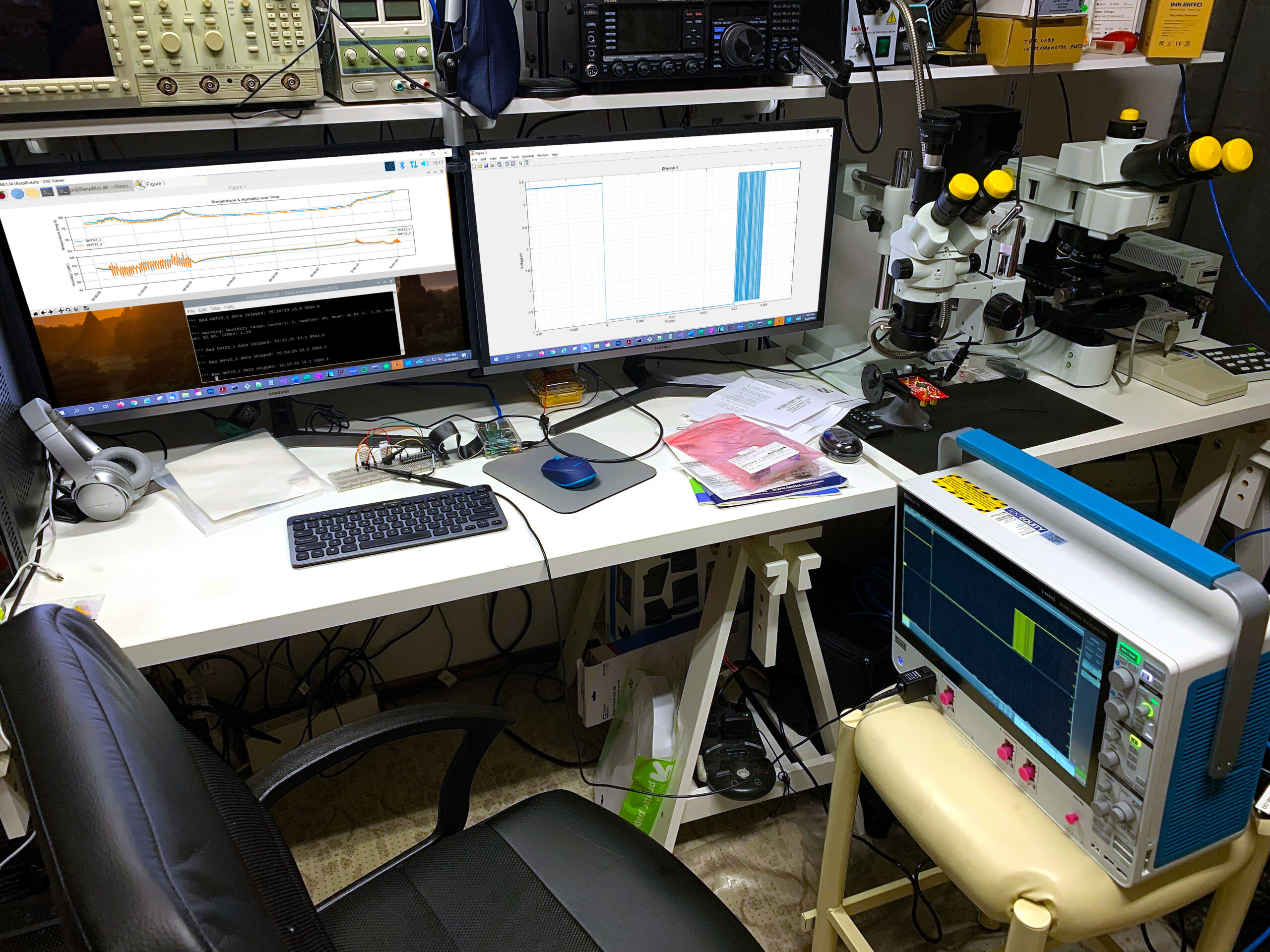
I am using a Raspberry PI 3 B+ to control 2 DHT22 temperature / humidity sensors along with Adafruit’s Python library. The circuit breadboard is shown on my lab bench in photo above. The photo shows the Tektronix MSO64 scope connected to the breadboard DHT22 output pin using a Tek TPP1000 passive probe. The scope channel 1 data is presented using the script presented later in this post on the right monitor. The output from the Raspberry PI’s 2 DHT22 sensors are shown on the left monitor. Not shown is the ethernet connection from scope to PC for MATLAB and e*scope remote control of the scope.

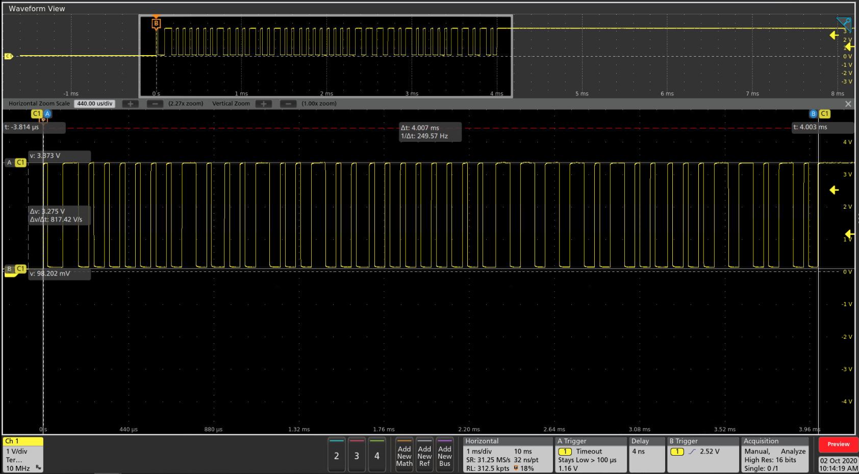
The e*scope screenshot presented below of the DHT22 sensor output looks just like the results on the scope itself. Click the photo to see a closeup of the pulse train from the sensor.

Results from using the script presented here

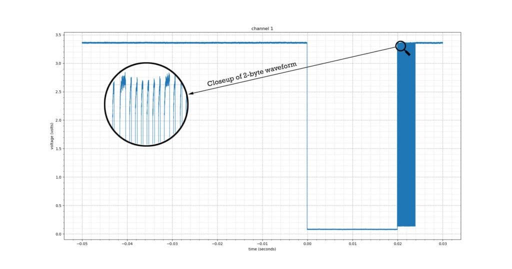
The photo below shows an example of 2-byte data capture to my PC. The noise level over-all seems normal to me using a passive probe connected to a working DHT22 Temperature Humidity output pin on a breadboard. The closeup shows a train of pulses of two width sizes. I think the tops of each pulse on closeup show signal noise of the 2-byte read process and is not internal to the DHT22 sensor. I base this conclusion on comparison to the e*scope screenshots shown in photo above. Further investigation in a future blog post will discuss the further investigation into the difference between the e*scope “square-like” signal vs the “ragged needs a hair cut” looking signal generated from the program captured “Curve?” data.

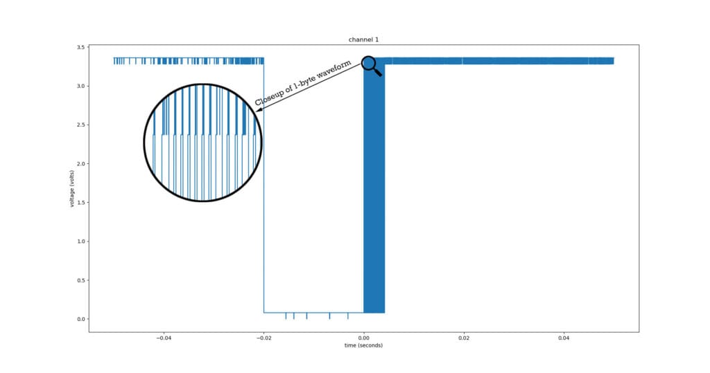
While the photo below shows what my 1-byte data capture MATLAB (or Python) scripts show using the same MSO64 scope. The noise level over-all seems large to me. The closeup shows a train of pulses of two width sizes. The tops of each pulse show data capture noise well beyond the signal internal to the DHT22 sensor and well beyond the 2-byte data capture presented in the MATLAB script here.

Description of the code

Use the MATLAB script below to capture and plot one channel of 2-byte data from your scope to your PC. I have made the script as short as possible to demonstrate the main principle of 2-byte data capture. It relies on MATLAB’s Instrument and Control Toolbox. In the initial comments I present a few discussion links showing other scripts that I learned from while developing this script. Yet each of these scripts have at least one problem making them unusable for me. Most use 1-byte data capture. The most promising script was the Oscilloscope App offered on MATLAB Central. But this script does not use trigger point relative to DATA:START for the waveform (PT_Off) so the plotted time base (X values) are not accurate.

The first lines of code are for initialization – including your scope’s address. I assume you have already installed VISA software on your PC. I use the National Instruments VISA software and driver with support for Windows and Mac OS via Ethernet, GPIB, serial, and USB. The bundled NI-MAX tool can be used to find the parameters you might need to configure the visa or gpib address in my script. Tektronix and Agilent also offer VISA software. MATLAB’s Instrument Tool Box offers the tmtool to list available driver details you can use to find your instrument’s visa or gpib address as well.

Throughout the code I use the old style transfer waveform preamble information WFMPRe commands instead of the more modern WFMOutpre commands. In this way, I am able to use this same script for my much older Tektronix TDS 784D scope with only one code change. This code change is implemented in lines 60 to 69 – just after the instrument identity request “*IDN?”.

Data acquisition if controlled through the use of the “DATa:ENCdq” command followed by “SRIbinary”. In this case we are reading 2-byte signed data in the range from -32,768 through 32,767 with byte order swapped  so the least-significant byte is transferred first “Little Endian Byte Order”.

The heart of the code is built around the binblockread(scope, ‘int16’) command and ‘CURV?’. If you are a python programmer than this command is similar to the python pyvisa library’s pyread_raw() function – which is not available in MATLAB. The code includes error checking with the scope’s “*esr” register. A value of 0 is returned when no error was found during the binary block read of data from the scope. Otherwise an error code and description results.

Scaling of time and waveform data is in the “%% Waveform and Time scaling” section of the code. The result will be Y-axis values in Volts, and X-axis values in Time. Because modern scopes often use pre-trigger settings, time will start at some negative value, not at 0.

%% MATLAB ICT: MSO64 / TDS 784 2-byte waveform read with plot
% Created on Wednesday Oct 6, 2020
% Updated on Thursday Oct 7, 2020
%
% Tested on both Tek MSO64 and TDS 784D scopes 
% (maybe many other scopes will work also - see lines 63 to 69 to add yours)
% 
% Referenced Discussion Threads:
%
%   MATLAB ICT: MDO Simple Plot
%   https://forum.tek.com/viewtopic.php?f=580&t=141809
%
%   MATLAB Oscilloscope App
%   https://www.mathworks.com/matlabcentral/fileexchange/69847-oscilloscope-app
%
%   Python MSO64 2-byte read binary waveform example
%   https://forum.tek.com/viewtopic.php?f=580&t=142410
%
%   Python: MDO Simple Plot
%   https://forum.tek.com/viewtopic.php?t=138684
%
% Author: BiophysicsLab.com

%% User Inputs
visa_vendor = 'NI'; 

% Uncomment and set one of these instrument access methods
gpib_board = 0; gpib_address = 14;
%visa_address = 'TCPIP0::192.168.1.32::inst0::INSTR';
%visa_address = 'USB0::0x0699::0x040C::QU000136::INSTR';

input_channel = 'CH1';

timeout = 5; % seconds
buffer_size = 3E6; % large enough to capture 2-byte int16 data

%% Initialize Instrument
% instrument connection config
if ~isempty(instrfindall)
    fclose(instrfindall);
    delete(instrfindall);
end

% Use GPIB or VISA
if exist('visa_address', 'var')
    scope = visa('NI', visa_address);
else
    scope = gpib('NI', gpib_board, gpib_address);
end
scope.InputBufferSize = buffer_size;
scope.OutputBufferSize = buffer_size;
scope.Timeout = timeout;

fopen(scope);

%% Instrument control
fprintf(scope,'*cls'); % clear ESR
fprintf(scope,'header OFF'); % disable attribute echo in replies

r = query(scope, '*idn?');
fprintf('%s\n', r);
% Old scopes need channel name in waveform parameter settings
if isletter(r(18))
    % Example: TEKTRONIX,TDS 784D,0,CF:91.1CT FV:v6.4e
    command_mod = input_channel;
else
    % Example: TEKTRONIX,MSO64,C012872,CF:91.1CT FV:1.22.4.7207
    command_mod = '';
end

% Record length settings
record = str2double(query(scope, 'HORizontal:RECORDLength?'));
fprintf(scope,'DATa:STARt 1');
fprintf(scope,['DATa:STOP '  num2str(record)]);

% Acquistion settings
fprintf(scope,['DATA:SOU ' input_channel]);
fprintf(scope,'DATA:WIDTH 2');
fprintf(scope,'DATA:ENC SRI');

%% Get waveform
fprintf(scope,'CURVE?');
data = binblockread(scope, 'int16');
% Tektronix scopes send and extra terminator after the binblock.
fread(scope, 1);

% error checking
r = query(scope, '*esr?');
fprintf('event status register: %s\n', strtrim(r));
r = query(scope, 'allev?');
fprintf('all event messages: %s\n', strtrim(r));
if isempty(data)
    error('binblockread: An error occurred while reading the waveform.');
end

%% Waveform and Time scale parameters
ymult = str2double(query(scope,['WFMPRE:' command_mod ':YMULT?']));
yzero = str2double(query(scope,['WFMPRE:' command_mod ':YZERO?']));
yoff = str2double(query(scope,['WFMPRE:' command_mod ':YOFF?']));

xincr = str2double(query(scope,['WFMPRE:' command_mod ':XINCR?']));
xzero = str2double(query(scope,['WFMPRE:' command_mod ':XZERO?']));
pre_trig_record = str2double(query(scope,['WFMPRE:' command_mod ':PT_OFF?'])); 

%% Close visa session
fclose(scope);
delete(scope);
clear scope;

%% Waveform and Time scaling

scaled_data = ((data - yoff) .* ymult) + yzero;

total_time = record * xincr;
t_start = (-1 * pre_trig_record * xincr) + xzero;
t_stop = t_start + total_time;
scaled_time = linspace(t_start, t_stop, record);

%% Plot
plot(scaled_time, scaled_data)
title('Channel 1')
xlabel('Time(s)')
ylabel('Voltage(V)')
xlim([t_start t_stop])
grid on
grid minor

fprintf('\nPlot complete\n')

Some References

• Updated version of this post with multichannel plotting
• NI-VISA (Virtual Instrument Software architecture) Help
• SCPI (Standard Commands for Programmable Instruments) commands
• MATLAB Instrument Control Toolbox
• Tektronix MSO64 Programmer Manual (release date 1/29/2021)
• Tektronix XYZs of Oscilloscopes – a primer