Short-time Fourier Transform

The STFFT technique is best suited for situations where the Fourier transform over the entire signal includes too many frequency artifacts from nonstationarities (statistical changes over time). Yet the technique also has its problems too. The 3-dimensional plot generated by STFFT is strongly affected by the windowing size used in the algorithm for example.

The goal of the Short-Time Fast Fourier Transform (STFFT) is to improve ability to interpret spectral features as they are changing over time.

Ron Fredericks, BiophysicsLab.com

STFFT Can Show Frequency Trends Over Time

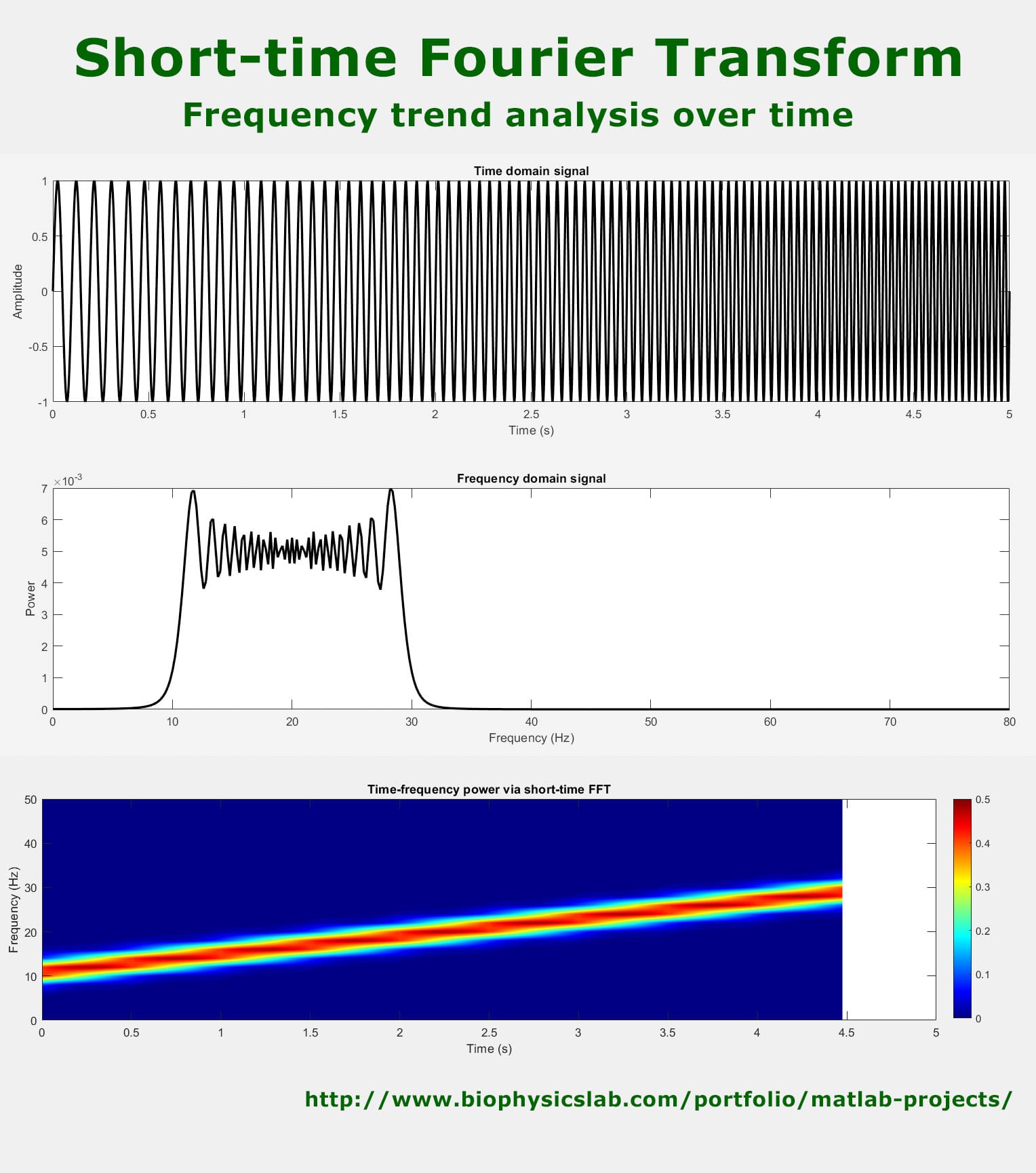
Figure 1: Top plot to the left shows a “chirp” signal that goes from 10 to 30 Hz over a 5 second time span. The resulting Fourier transform is shown in the middle plot. The power vs frequency result is not too helpful in explaining the trend over time shown in the original signal (top plot). The bottom plot shows the result of Short-time Fast Fourier transform (STFFT). It produces a color encoded result clearly showing the frequency power level trend over time in the “chirp” signal. Note that x-axis is the time, y-axis is the frequency, and the z-axis is a color encoded power level from each 25 ms time size taken 500 ms at a time.

Four steps are required for a short-time FFT example.

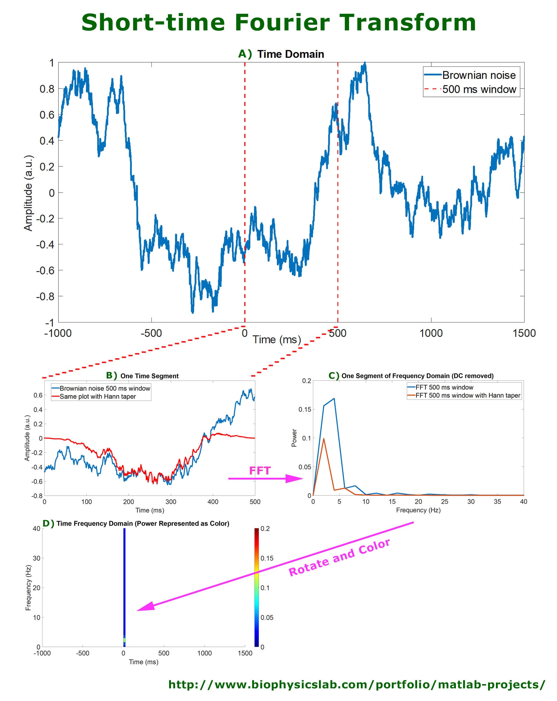
• A) Upper plot shows a signal with singularities.
• B) Middle left plot shows one 500 ms segment of the signal along with result of dot product with Hann taper.
• C) Middle right shows the FFT for just this one-time segment.
• D) Lower left shows the first 500 ms FFT segment rotated and colored to show time, frequency, and power (using colorbar).
• The process would be repeated moving the 500 ms slice one 25 ms increment to the right at a time. The resulting color-coded signal can show how FFT changes over time.
• See MATLAB results below for an example.

STFFT Window Size Increases Time or Frequency Resolution

Wikipedia’s Short-time FFT Example discusses the problem behind selection of window size. When the window size is small, the signal time changes are enhanced for accurate measurement. When the window size is larger, the frequency over time is enhanced for accurate measurement. What follows here is MATLAB code developed to demonstrate this Wikipedia example.

The plots below compare the STFFT method using three different Hann taper window sizes from 25 ms to 500 ms. At 25 ms, the time change is best displayed. The transitions are clear and easy to measure at 5, 10 and 15 seconds. At 500 ms, the frequency change is best displayed. The frequencies from 2 to 8 Hz are easy to measure.

MATLAB Code

Below is my MATLAB code demonstrating the Wikipedia STFFT time window issue for enhanced time or frequency analysis. Additional discussion can be found in my MATLAB notes: lesson 43 – Solutions to understanding nonstationary time series located in my published notes MASTER THE FOURIER TRANSFORM AND ITS APPLICATIONS

%% Demonstrate Short-time FFT using MATLAB
%     Following Wikipedia Example
%     https://en.wikipedia.org/wiki/Short-time_Fourier_transform#Example
%
% Follow STFFT code structure taught by Dr. Mike X Cohen
%     Lecture 43. Solution to understanding nonstationary time series
%     https://www.udemy.com/course/fourier-transform-mxc/
%
% Developer: BiophysicsLab.com
%

% simulation details
fs     = 400; % sampling rate
time   = 0:1/fs:20; % time line

% create signal with several frequency non-singularities
f      = [2 4 6 8]; % frequencies in Hz
ft     = [0,5;  5,10; 10,15;  15,20]; % time intervals for each f
signal = [];
for fi = 1: size(ft,1)
    signal = [signal  ...
        cos( 2*pi.*f(fi).*time( time>=ft(fi,1) & time<ft(fi,2) ) )];
end

%% Plot signal amplitude vs time and power vs frequency
figure(1), clf

% plot Signal vs Time
subplot(211)
plot(time(1:end-1),signal,'k','linew',2)
xlabel('Time (s)'), ylabel('Amplitude')
title('Time domain signal')

% compute power spectrum
npnts  = length(time);
sigpow = 2*abs(fft(signal)/npnts).^2;
hz     = linspace(0,fs/2,floor(npnts/2)+1);

% plot Power vs Frequency
subplot(212)
plot(hz,sigpow(1:length(hz)),'k','linew',2)
xlabel('Frequency (Hz)'), ylabel('Power')
set(gca,'xlim',[0 20])
title('Frequency domain signal')

%% short-time FFT
% demonstrate frequency vs time resolution using 3 seperate window lengths
figure(2), clf

subplot(311)
winlen   = 30; % window length for STFFT for improved time resolution
stepsize = 25;  % step size for STFFT
[tf1,numsteps1,hz1] = shortTimeFFT(fs,signal,time,winlen,stepsize);

subplot(312)
winlen   = 150; % window length for STFFT
stepsize = 25;  % step size for STFFT
[tf2,numsteps2,hz2] = shortTimeFFT(fs,signal,time,winlen,stepsize);

subplot(313)
winlen   = 500; % window length for STFFT for improved frequency resolution
stepsize = 25;  % step size for STFFT
[tf3,numsteps3,hz3] = shortTimeFFT(fs,signal,time,winlen,stepsize);


%% Short-time FFT local function

function [tf,numsteps,hz] = shortTimeFFT(fs,signal,time,winlen,stepsize)
% shortTimeFFT 
%   impliments Short-time FFT algorithm
%   plots results using MATLAB contourf function
%
% INPUT
%     fs: sample rate
%     signal: vector holding signal data
%     time:  vector holding time data (same length as signal vector)
%     winlin: length of time window for Short-time FFT calculations
%     stepsize: length of each step during frequency-time loop
%
% RETURN
%     tf: matrix holding time frequency results
%     numsteps: number of steps used to create tf
%     hz: vector holding the frequency for each step in tf

    % plot controls
    ylims = [0 10]; % frequency range
    xlims = [0 20]; % time range
    clims = [0 .5]; % Power colorbar range

    npnts  = length(time);
    numsteps = floor( (npnts-winlen)/stepsize );
    hz = linspace(0,fs/2,floor(winlen/2)+1);

    % initialize time-frequency matrix
    tf = zeros(length(hz),numsteps);

    % Hann taper
    hwin = .5*(1-cos(2*pi*(1:winlen) / (winlen-1)));

    % loop over time windows
    for ti=1:numsteps

        % extract part of the signal
        tidx    = (ti-1)*stepsize+1:(ti-1)*stepsize+winlen;
        tapdata = signal(tidx);

        % FFT of these data
        x = fft(hwin.*tapdata)/winlen;

        % and put in matrix
        tf(:,ti) = 2*abs(x(1:length(hz)));
    end

    % plot
    contourf(time( (0:numsteps-1)*stepsize+1 ),hz,tf,40,'linecolor','none')
    set(gca,'ylim',ylims,'xlim',xlims,'clim',clims)
    xlabel('Time (s)'), ylabel('Frequency (Hz)')
    title(['Time Frequency Power: Hann taper Short-time FFT with ' num2str(winlen) ' ms window']);
    colorbar

end