RC and RL Circuit Simulation
Table of Contents
MATLAB simulator for RC and RL circuits
My utility for the display and reuse of RC and RL circuit simulations in MATLAB is presented here. I offer both a GUI and a command line version running from the same code base. I envision this application to be useful in both electronics teaching and in lab design environments. The interactive MATLAB GUI allows the user to quickly appreciate the symmetry between curves generated for 8 combinations of RC and RL circuits using the Circuit (Resistor/Capacitor or Resistor/Inductor), Parameter (Voltage or Current), and Switch S1 (Charge or Discharge) buttons. While the command line version offers more nuanced control over parameters with the same plots and plugins offered by the GUI.
Both GUI and constructor versions require MATLAB version 2020a or newer. The code runs on all MATLAB-supported platforms: Windows, Mac, and Linux platforms.
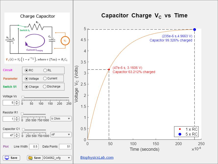
Figure 1 above shows the interactive GUI interface using MATLAB’s “App Designer“.
Simulation integrated with Flexible Output Plugins
Example plugins included with this code release allow arbitrary waveforms to be generated for breadboard circuit design. The user can compare the live breadboard RC and RL components with the same circuit in simulation using a multi-channel oscilloscope and a waveform generator – or – from Excel spreadsheet output. Each of the plugins are offered from the “save” icon
Also, the user can add their own plugins for other uses or models of Arb wave generator following the examples provided in the plugins subdirectory. All scripts in the plugin directory show up as selections in the save feature’s “pull-down” option near the bottom of the GUI or as a parameter in the constructor non-GUI version. Additional plugin scrips would show up in this same GUI pull-down menu or be available to the constructor as well.
Simulation integrated with Excel Spreadsheet
- Excel spreadsheet: RC_RL_plot_support_files\plugins\ExcelFile.m
Simulation integrated with Arbitrary Waveform Generator
A unique feature offered by this simulation is the ability to interface the RC RL plot data to custom plugins. Students, engineers, or scientists may find the existing plugin scripts useful:
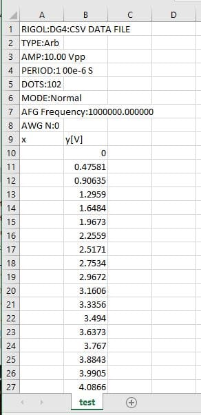
- CSV data file to generate RC RL curves using a RIGOL D4062 AWG Waveform Generator: RC_RL_plot_support_files\plugins\DG4062_wfg.m
- CSV data file to generate RC RL curves using the Tektronix MSO 3,4,6 series AWG Function Generator: RC_RL_plot_support_files\plugins\MSO64B_afg.m
I include notes on the format for many other RIGOL AWG waveform generators:
- RC_RL_plot_support_files\notes\RIGOL ARB File Format
Programming Notes.
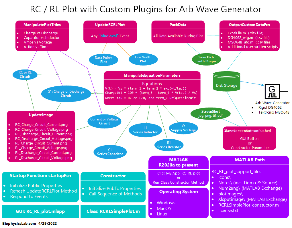
I designed the code from MATLAB’s App Designer which enforces an OOP methodology. The key methods are highlighted in the diagram below “RC / RL Plot with Custom Plugins for Arb Wave Generator” Figure 3. The source code for both the GUI and nonGUI versions of the code can be found in the notes section of the support files included in this package.
Simulation without GUI using the class constructor
For those that prefer to run their MATLAB projects as a script, I include a non-GUI constructor that uses the same codebase, properties, and methods from the GUI codebase. The constructor script can be found in the installed code base: RCRLSimplePlot_Constructor.m.
Code for the constructor is shown below along with comments explaining the use for each parameter. Where each parameter calls the same methods as in the event-driven GUI.
% RCRLSimplePlot(RC_circuit, charge_circuit, current_circuit, Vs, R1, C1, L1, data_pnts, line_width, plugin_name, save_screen)
RCRLSimplePlot(true, true, true, 5, 5e6, 5e-6, 5e-3, 51, 0.5, "ExcelFile", true);

%% Notes

% RC_circuit is a boolean value. Icons for each of the 8 combinations of
% circuit are located in the icons\ subdirectory as png and vsdx (Visio) files.
%
%     true               Project is a resistor / capacitor RC circuit (so L1
%                        value will be ignored).
%     false              Project is a resistor / inductor RL circuit (so C1
%                        value will be ignored).
%
% charge_circuit is a boolean value.
%
%     true               Project has S1 switch in the circuit set to charge.
%     false              Project has S1 switch in the circuit set to discharge.
%
%
% current_circuit is a boolean value.
%
%     true               Project plots current vs time
%     false              Project plots voltage vs time
%
%
% Vs is a floating point number defining supply voltage (in volts).
%
%
% R1 is a floating point number defining the series resistor in the circuit
% (in Ohms).
%
%
% C1 is a floating point number defining the series capacitor in the circuit
% (In Farads). Value not used in RL circuits. (RC_circuit = true).
%
%
% L1 is a floating point number defining the series inductor in the circuit
% (In Henrys). Value not used in RC circuits. (RC_circuit = false).
%
%
% data_pnts is a positive integer greater than or equal to 2. The number
% defines how many data points will be used in both the plot and in the
% plugin scripts.
%
%     For Rigol DG4062 script DG4062_wfg.m, the maximum data points can be
%     1024*16/2 or 8192. Divided by 2 because the arbitrary curve includes
%     both a charge (or discharge) plus a zero padded flat line of the same
%     length. Thus the full arb wave generated will fit into a square wave with
%     a period of 5*tau.
%
%     For Tektronix MSO64b script MSO64B_afg.m, the maximum data points can be
%     1024*128/2 or 65536. Divided by 2 because the arbitrary curve includes
%     both a charge (or discharge) plus a zero padded flat line of the same
%     length. Thus the full arb wave generated will fit into a square wave with
%     a period of 5*tau.
%
%
% line_width is a small floating point number typically in the range of 0.5 to
% 10. The number defines the width of the plotted line.
%
%
% plugin_name is a script name (without .m) in the plugins subdirectory,
% (be careful for correct capitalization). Use "none" to skip this feature.
% I envision the two Arb instrument scripts to be used to display the
% circuit charge or discharge curve on an oscilloscope along with the
% actual results of a breadboarded circuit powered with a square wave. See
% link below for a blog post demonstrating this usage.
% Scripts include:
%
%       none                    Skip the Plugin save feature
%
% 	ExcelFile		Script to save RC_RL_plot app curve results for
% 						saving results in XLSX Excel file format. Windows PC ActiveX
% 						offers more features so on the PC plot and circuit
% 						images are embedded into the Excel file.
%
% 	DG4062_wfg		Script to save RC_RL_plot app curve results for
% 						Rigol DG4062 wave form generator in csv format.
% 						See the notes\ subdirectory for details on how to
% 						configure this output for other Rigol wfg instruments.
%
% 	MSO64B_afg 	        Script to save RC_RL_plot app curve results for
% 						Tektronix MSO64B Oscilloscope's licensed arbitrary wave
% 						generator in CSV format. The same CSV format should work
% 						for other Tektronix MSO (4, 5, and 6) series scopes with a
% 						licensed afg.
%
%
% save_screen is a boolean value.
%
%     true              Present dialog to save plot screen as .jpg, .png,
%                       .tif, or .pdf image.
%     false             Screen save option will be skipped.

%% Reference link:

% Arbitrary Wave Generator Compliments MATLAB RC and RL Circuit Simulation
% https://www.biophysicslab.com/2022/04/27/arbitrary-wave-generator-compliments-matlab-rc-and-rl-circuit-simulation/
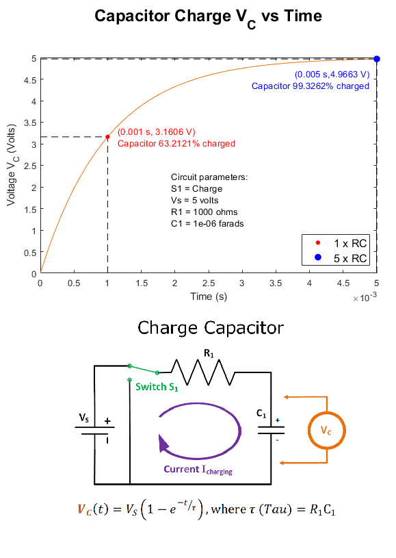
The plot output from the constructor looks similar to what is provided in the GUI version.
RC and RL charge/discharge equation management
For MATLAB code development I start with the basic equation for voltage change over time for RC circuit.
 ~=~ V_S(1- e^{-t/tau})")

Then I add general terms (term_x) to control the circuit for all 8 configurations of charge/discharge RC/RL, and Voltage/Current. What I came up with was two categories to represent all 8 configurations with each of the terms in term_x being very simple such as 0, 1, -1. See code below.
function ManipulateEquationParameters(app)

            % Descriptions of truth table parameters
            %
            %   Charge, or discharge equation parameters:
            %       V @ t = Vs * (app.term_1 + app.term_2 * exp(-t/tau));
            %
            %   Percent charge, or discharge equation parameters:
            %       Percent @ 1*tau = 100 * (app.term_3 + app.term_4 * V@tau / Vs)
            %       Percent @ 5*tau = 100 * (app.term_3 + app.term_4 * V@5tau / Vs )
            %
            %   Where:
            %       t is time in seconds
            %       V is instantaneous Voltage (or current)
            %       Vs is constant circuit supply voltage (or current)
            %       tau = R*C (or L/R) measured in seconds
            %       R, C, L: Resistor (ohms), capacitor (Farads), inductor (Henry) circuit value
            %
            %   Small offset for 5RC or 5RL display: app.adj_str_5rcx and app.adj_str_5rcy
            %
            %   Optimized placement of 5RC (or 5RL) text: app.pcnt_txt_on_bottom
            %
            %   Optimized placement of time constant legend: app.lgndPosition

            if (app.RCButton.Value && app.ChargeButton.Value && app.C_T_Button.Value) ||...
               (app.RCButton.Value && ~app.ChargeButton.Value && ~app.C_T_Button.Value) ||...
               (~app.RCButton.Value && ~app.ChargeButton.Value && app.C_T_Button.Value) ||...
               (~app.RCButton.Value && app.ChargeButton.Value && ~app.C_T_Button.Value)
                % Truth Table for decay waveforms: e^(-x)
                %   RC Discharge Voltage
                %   RC Charge Current
                %   RL Charge Voltage
                %   RL Discharge Current
                app.term_1 = 0;
                app.term_2 = 1;
                app.term_3 = 1;
                app.term_4 = -1;
                app.pcnt_txt_on_bottom = false;  % Display percent charged
                                                 %   info as first line of
                                                 %   text.
                app.adj_str_5rcx = -.02;   % Tweek data point display text
                app.adj_str_5rcy =  .12;   %   above 5RC (or 5RL).

                app.lgndPosition = ["Location","northeast"];

            else
                % Truth Table for growth waveforms: 1-e^(-x)
                %   RC Charge Voltage
                %   RC Discharge Current
                %   RL Discharge Voltage
                %   RL Charge Current
                app.term_1 = 1;
                app.term_2 = -1;
                app.term_3 = 0;
                app.term_4 = 1;
                app.pcnt_txt_on_bottom = true;  % Display percent charged
                                                %   info as second line of
                                                %   text.
                app.adj_str_5rcx = -.02;  % Tweek data point display text
                app.adj_str_5rcy = -.04;  %    below 5RC (or 5RL).

                app.lgndPosition = ["Location","southeast"];

            end
        end
Plugin Script Details
Excel File Output using the Excel file plugin script
Saving data using the “ExcelFile” plugin is easy from the pull-down and save button on the GUI, or by selecting “ExcelFile” from the constructor option.
The results from the “ExcelFile” plugin are shown below as a PDF just so it was easier to display on this web page. The actual output looks just like this, only in .XLSX format. The Windows version of the script includes ActiveX support so I place the plot and circuit images into the excel file as shown in the pdf display below. While the Linux and macOS versions of the excel file will not have these images.
PDF File TODO
CVS File Output using the DG4062_awg plugin script
This script is used to format plot results for upload to a RIGOL DG4062 Arbitrary Wave Generator Instrument. The CVS file is copied to a USB memory stick and then transported to the RIGOL instrument using its USB port. The curve output from the arbitrary wave option will then look like the plotted curve in the MATLAB simulator.
Details are included in the notes subdirectory to change the titles in the first 8 lines so the CSV file will be accepted by other Rigol WFG instruments. These changes could be made in a separate copy of the Rigol DG4062_awg plugin script or manually changed in the existing CSV file.
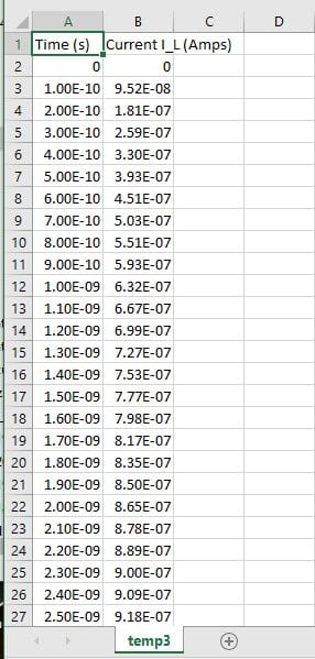
CVS File Output using the MSO64B_afg plugin script
This script is used to format plot results for upload to a Tektronix Arbitrary Frequency Generator included within a TEK MSO64B Oscilloscope. The file is copied to a USB memory stick and then transported to the Tek scope instrument using its USB port. The curve output from the arbitrary wave option will then look like the plotted curve in the MATLAB simulator.
The default data points for plotting are set to 51. The number of data points should be increased significantly to improve the Arb wave output. Unlike the Rigol WFG instrument, the interpolation between datapoints in the Tektronix AFG produces a staircase curve that is not very smooth. Increasing the number of plotted data points (and therefore the number of data points sent to the AFG instrument) can produce a much smoother curve for display on the oscilloscope.
Installation
Note: RC_RL_Plot runs correctly on MATLAB Windows, MacOS, and Linux version 2020a and above .
Installation steps:
- Download the install file linked below.
- Right-click the unzipped install file: RC_RL_plot.mlappinstall.
- Select install to put script and support files into place for MATLAB.

MATLAB RC_RL_plot
9
2026-05-03 14:35:50 GMT
Steps to launch app:
- Open MATLAB, select APPS tab near upper left.
- Select more apps using the down arrow near the upper right, and click on RC_RL_plot app in the “My Apps” area.
- The RC_RL_plot app will open a window similar to Figure 1 after what seems like a long time (5 seconds on my machine).
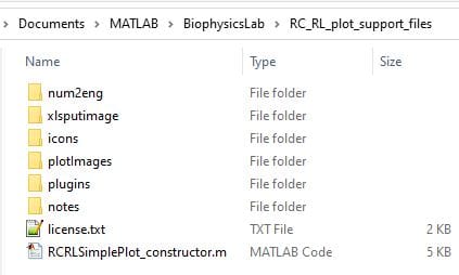
Support files
If you install this code following the install app procedure as shown in this article. The support files will be placed into the MATLAB path as shown in the figures below