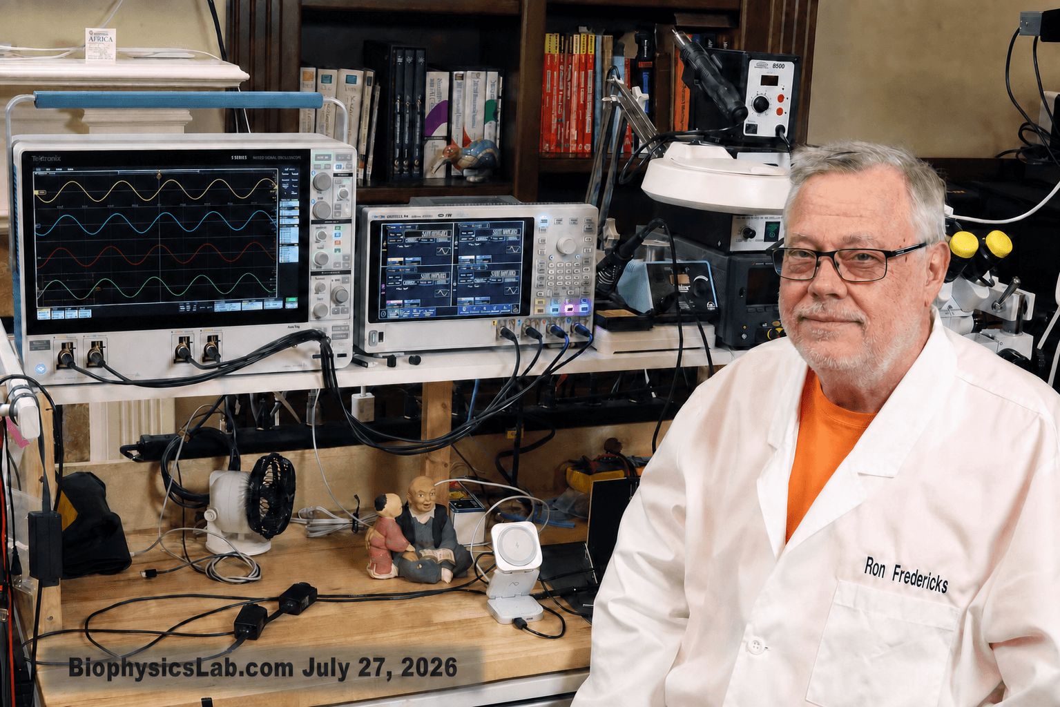
DG5254 Pro Waveform Generator – Introduction
The Rigol DG5000 Pro family can accept newline-terminated SCPI commands through a raw TCP socket. These demonstrations use MATLAB’s tcpclient object or Python’s socket.create_connection. They do not require a VISA layer.
There are two reusable products in this project: tested MATLAB and Python starter code for controlling a Rigol DG5000 Pro, and a human-directed AI workflow for developing stronger MATLAB code through repeated cycles of context, execution, measurement, and reflection—a process I call Cycles of Efficiency™.
The project began with the practical goal of creating readable, reusable instrument-control examples. The DG5000 Pro is a relatively new series: Rigol introduced the original two-channel models in 2024 and expanded the family with four- and eight-channel models in July 2025. Public searches tend to lead to product pages and programming manuals rather than complete, experimentally verified MATLAB examples, so this article fills a useful gap without claiming to be the first. During code development and preparation of the article, a second goal emerged: create portable project context that helps an AI coworker understand advanced MATLAB methods, work under human direction, compare requested settings with instrument read-back and oscilloscope measurements, and carry validated lessons into future projects.
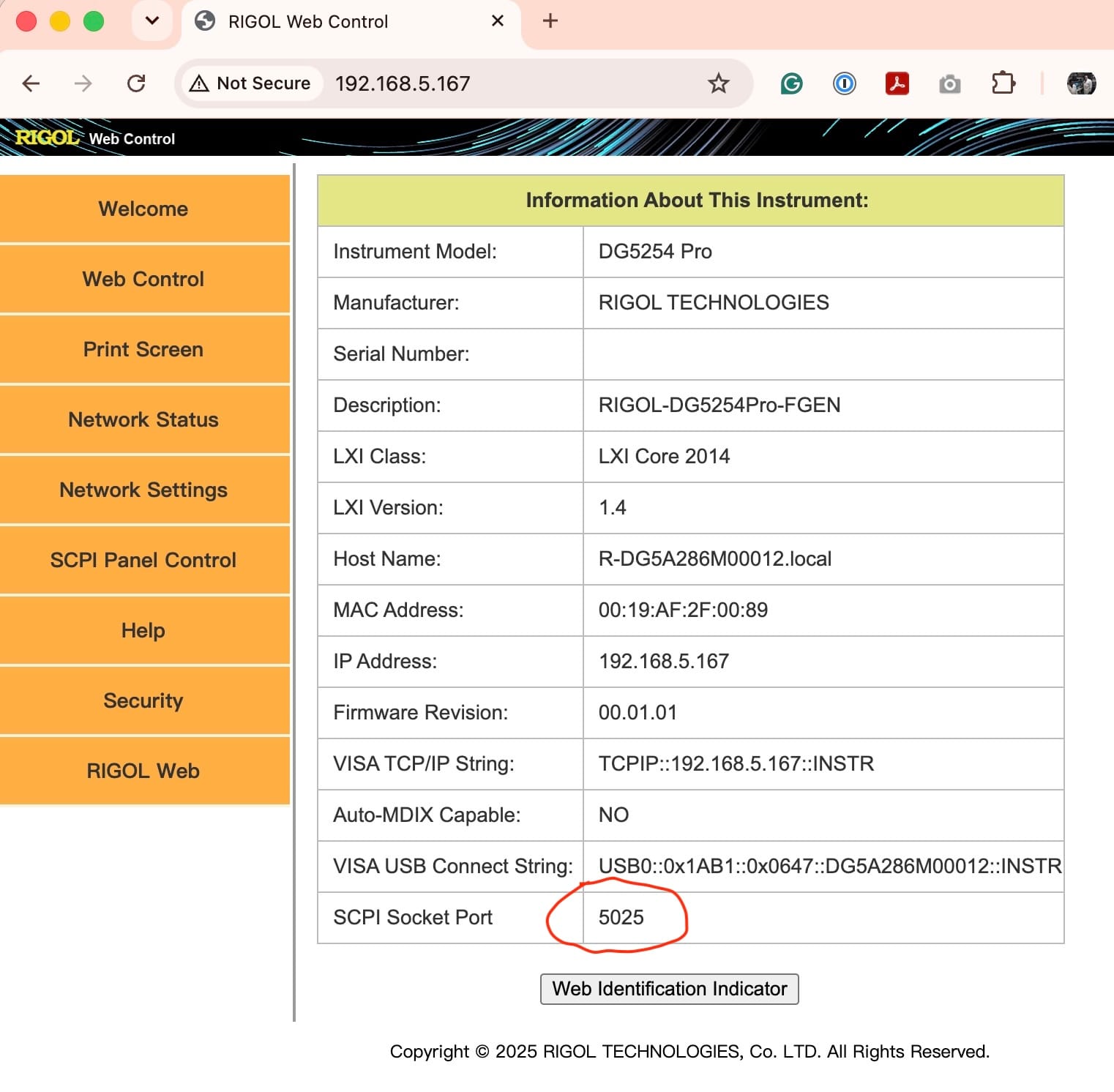
A raw SCPI socket sends newline-terminated commands directly to a TCP port selected by the instrument. VXI-11 carries instrument commands through a different RPC-based network service and does not use that same raw-socket connection. Rigol models may support one or both transports, and the available raw-socket port can vary by instrument and configuration. Therefore, do not copy port 5025 merely because it works in this example; use the SCPI Socket Port reported by your instrument. This DG5254 Pro reports port 5025 on its own web Welcome page, so that is the port used below.
The article starts with network setup and two small identification examples—Python on Channel 1 and MATLAB on Channel 2—then develops a MATLAB demonstration that configures, reads back, and phase-aligns selected channels on 2-, 4-, or 8-channel DG5000 Pro models. The analog results were observed on a Tektronix MSO64B.
Want the files first? Jump directly to the Project Download for the tested MATLAB and Python scripts, documentation, and reusable AI-context files.
The following table lists the Rigol DG5000 Pro AWGs that this code base is designed to support. Hardware testing for this article was performed on the four-channel DG5254 Pro; users of other models should confirm commands and limits against their instrument documentation.
Model | Max Frequency | Channels |
|---|---|---|
DG5252 Pro | 250 MHz | 2 |
DG5254 Pro | 250 MHz | 4 |
DG5258 Pro | 250 MHz | 8 |
DG5352 Pro | 350 MHz | 2 |
DG5354 Pro | 350 MHz | 4 |
DG5358 Pro | 350 MHz | 8 |
DG5502 Pro | 500 MHz | 2 |
DG5504 Pro | 500 MHz | 4 |
DG5508 Pro | 500 MHz | 8 |
Find and Preserve the Network Settings
Before running either script, identify the instrument’s current IP address and the raw SCPI socket port reported by that instrument.
Find the instrument’s IP address
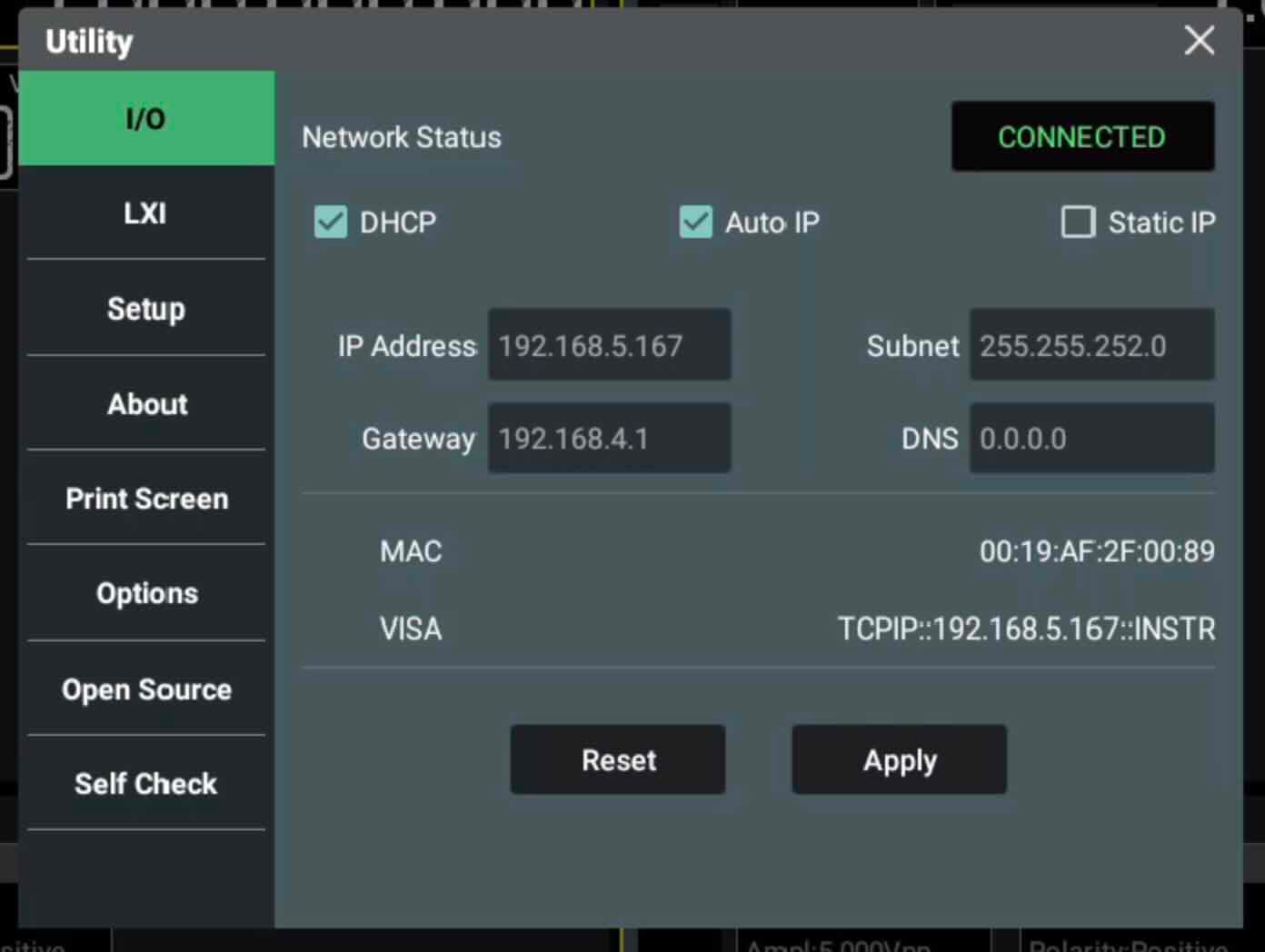
On the DG5000 Pro, open Utility > I/O to view the current IP address and whether the network is using DHCP or a static address.
Keep a DHCP address consistent
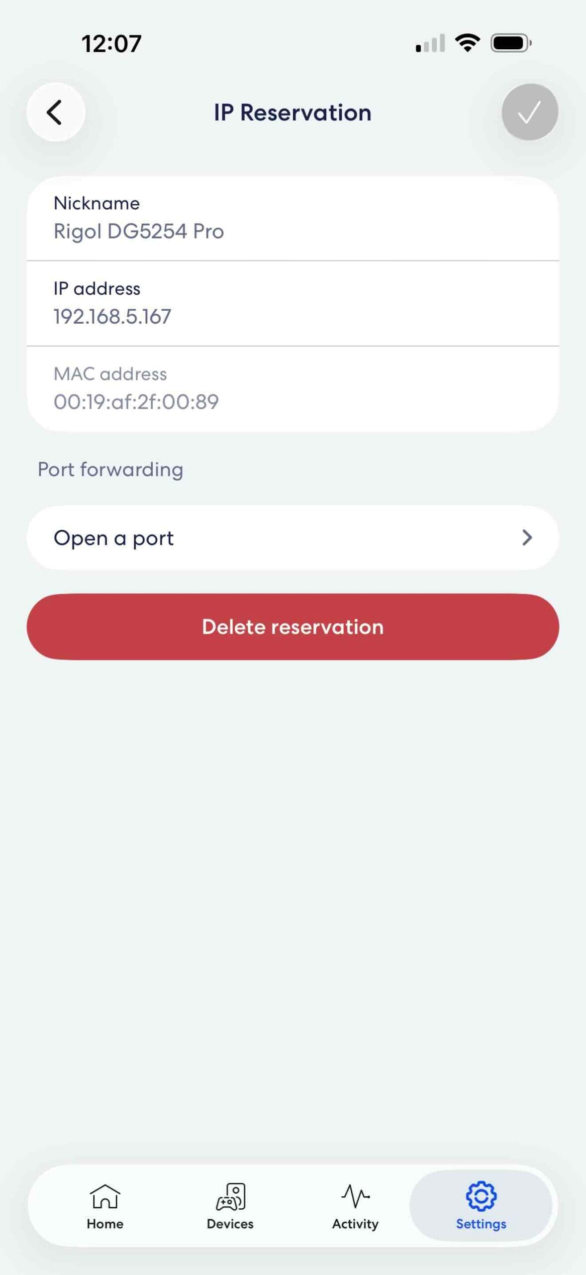
I leverage my router’s DHCP IP-reservation feature rather than configure a static IP address on the instrument. On my eero router, I open Settings > Advanced networking > Reservations & port forwarding, find the instrument by its IP and MAC addresses, and reserve that address. The router can then return the same address whenever the generator reconnects.
Read the SCPI socket port from the instrument
Open the instrument’s IP address in a web browser to discover the port number. The Welcome page identifies the model, firmware, IP address, and SCPI Socket Port. Use that displayed port in the code. In this example the value is 5025.
Minimal Driverless MATLAB and Python Examples
The two starter examples use deliberately different outputs so they can run together and be distinguished during validation. Python configures Channel 1 for a 5 kHz, 2 Vpp sine wave; MATLAB configures Channel 2 for a 7 kHz, 1.5 Vpp sine wave. Both use a HighZ load setting, query *IDN?, enable their respective output, and close the TCP connection. Closing the connection does not disable either waveform.
MATLAB Starter Code: Channel 2
Some code highlights: writeline adds the configured LF terminator. The catch block releases a connection that was created and then rethrows MATLAB’s original exception, preserving its identifier and stack trace.
% --- MATLAB Driverless Control for Rigol DG5254 Pro ---

% Initialize the connection variable so the catch block can safely inspect it
device = [];

% 1. Define the Instrument's LAN Parameters
rigolIP = '192.168.5.167'; % <-- Replace with your generator's actual IP
rigolPort = 5025;          % <-- Use the SCPI Socket Port shown by your Rigol

try
    % 2. Open a direct TCP link (No VISA required)
    % Set a 3-second timeout for safe network response handling
    device = tcpclient(rigolIP, rigolPort, 'Timeout', 3.0);

    % Rigol RAW SCPI commands use a line-feed terminator
    configureTerminator(device, "LF");

    fprintf('Connected successfully to Rigol DG5254 Pro at %s:%d!\n', ...
        rigolIP, rigolPort);

    % 3. Query the Instrument Identification (*IDN?)
    % writeline automatically adds the configured newline character (\n)
    writeline(device, '*IDN?');

    identity = strtrim(readline(device));
    fprintf('Instrument ID: %s\n\n', identity);

    % 4. Match a 1 Mohm oscilloscope input, then configure Channel 2 for a
    % 7 kHz, 1.5 Vpp sine wave with zero offset and phase
    disp('Configuring Channel 2...');
    writeline(device, ':OUTPut2:LOAD INFinity');
    writeline(device, ...
        ':SOURce2:APPLy:SINusoid 7000,1.5,0.0,0.0');

    % 5. Example: Turn the Channel 2 Output ON
    writeline(device, ':OUTPut2:STATe ON');
    disp('Channel 2 output is now enabled.');

catch ME
    % Release the TCP connection if it was successfully created
    if ~isempty(device)
        clear device
    end

    % Preserve and reissue the original exception with its stack trace
    rethrow(ME);
end

% 6. Close the direct TCP connection after successful completion
clear device
disp('Rigol TCP connection closed; Channel 2 remains enabled.');The command sequence now packaged in the MATLAB starter produced no Code Analyzer error or warning messages in MATLAB R2026a and was live-verified on a DG5254 Pro on August 22, 2026. Codex in the ChatGPT desktop app used user-approved Computer Use to operate the MATLAB desktop, while MATLAB connected directly to the Rigol over TCP. Ron confirmed the resulting 7 kHz, 1.5 Vpp Channel 2 waveform on the Tektronix MSO64B.
During live verification, the earlier Python-controlled Channel 1 waveform remained at 5 kHz and 2 Vpp while MATLAB configured Channel 2. The Rigol read back 7000 Hz, 1.5 Vpp, and output state 1 for Channel 2, and the Tektronix MSO64B independently measured 7 kHz and 1.5 Vpp. Those distinct outputs made it immediately clear which language controlled each channel.
Python Starter Code: Channel 1
Some code highlights: The query helper reads until the terminating newline rather than guessing a response-buffer size. Nested context managers close both the text reader and socket after normal completion or an exception.
import socket


def send_scpi(device, command):
    # Send one newline-terminated SCPI command.
    device.sendall(f"{command}\n".encode("ascii"))


def query_scpi(device, reader, command):
    # Send a SCPI query and read through its terminating newline.
    send_scpi(device, command)

    response = reader.readline()

    if response == "":
        raise ConnectionError(
            f"The Rigol closed the connection while answering {command!r}."
        )

    return response.rstrip("\r\n")


rigol_ip = "192.168.5.167"
rigol_port = 5025
timeout = 3.0

try:
    # Both context managers close automatically after success or an error.
    with socket.create_connection(
        (rigol_ip, rigol_port), timeout=timeout
    ) as device:
        with device.makefile(
            "r", encoding="ascii", newline="\n"
        ) as reader:
            identity = query_scpi(device, reader, "*IDN?")
            print(f"Instrument ID: {identity}")

            send_scpi(device, ":OUTPut1:STATe OFF")
            print("Channel 1 output turned off.")

            # Match the 1 Mohm input used by a typical oscilloscope channel.
            send_scpi(device, ":OUTPut1:LOAD INFinity")

            send_scpi(
                device,
                ":SOURce1:APPLy:SINusoid 5000,2.0,0.0,0.0",
            )
            print(
                "Channel 1 configured: "
                "5 kHz, 2.0 Vpp, 0.0 V offset, 0 degrees."
            )

            send_scpi(device, ":OUTPut1:STATe ON")
            print("Channel 1 output turned on.")

    print("TCP connection closed; Channel 1 remains enabled.")

except Exception as exc:
    print(f"Rigol communication failed: {exc}")
    print(f"Exception type: {type(exc).__name__}")
raiseVerified Python output
This output was captured from a successful DG5254 Pro run on August 22, 2026. Codex in the ChatGPT desktop app used user-approved Computer Use to operate the Python environment, while the Python socket connected directly to the Rigol over TCP. Ron confirmed the resulting 5 kHz, 2 Vpp Channel 1 waveform on the Tektronix MSO64B. The serial-number field is redacted, and Channel 1 remains enabled after the connection closes.
$ python3 DG5254Pro_First_Script_Show_IDN_Start_Ch1.py
Instrument ID: RIGOL TECHNOLOGIES,DG5254 Pro,DG5A286Mxxxxx,00.01.01
Channel 1 output turned off.
Channel 1 configured: 5 kHz, 2.0 Vpp, 0.0 V offset, 0 degrees.
Channel 1 output turned on.
TCP connection closed; Channel 1 remains enabled.A Tektronix MSO64B also measured the resulting Channel 1 waveform at 5 kHz and 2.0 Vpp, independently confirming that the Python-controlled output reached the oscilloscope with the requested frequency and amplitude.
MATLAB Demonstration for Up to Eight Sine-Wave Channels
The main demonstration keeps the top-level flow readable by moving repeated work into local functions, following the structured and reusable coding methods highlighted in the MATLAB course-note references provided with this project. Its 8-by-6 numeric matrix contains channel number, enable flag, frequency, amplitude, phase, and expected load. Rows with Enable equal to zero are ignored, so their remaining values may be zero or retain useful values for future reuse; those values are not written to the instrument until the row is enabled.
- Validate the matrix shape and the selected model’s maximum channel count before connecting.
- Turn off only the selected outputs; unselected output states remain unchanged.
- Write load, frequency, amplitude, and phase for every selected channel.
- Read those stored settings back and compare them with the requested values.
- Enable outputs only after all selected channels pass read-back verification.
- If the selected phase-reference channel is active, build the Rigol bundle and perform one-shot phase alignment.
The read-back feature proves that the generator accepted and stored the requested settings. It does not measure the analog waveform at the connector or at the device under test; the oscilloscope provides that independent check. However, read-back provides a compact programmatic validation of all stored settings without requiring the user to query and inspect each parameter manually.
MATLAB Multichannel Demonstration Code
% File: DG5000Pro_MultiChannel_Sine_Demo.m
%
% Developed by BiophysicsLab.com
% Last revision date: August 22, 2026
%
% Overview:
% MATLAB Multi-Channel Sine Wave Control Script for Rigol DG5000 Pro AWG
% Ethernet via tcpclient object without VISA or Instrument Control Toolbox
%
% Purpose:
% Starter code for MATLAB users to test DG5000 Pro series AWGs and build
% more advanced control.
%
% Program flow:
%  1. Configure
%       - IP address and port number,
%       - Instrument maximum channel count,
%       - Instrument control matrix:
%           + Channel number,
%           + Channel control flag (1 yes, 0 ignore),
%           + Sine parameters: voltage, frequency, and phase,
%           + Expected load impedance in ohms, or Inf for HighZ,
%       - Phase-reference channel or 0 to disable phase align feature.
%  2. Test that the channel configuration is numeric and 8-by-6.
%  3. Check that no channel beyond max_allowed is selected.
%  4. Extract the active channel configuration once.
%  5. Connect to and identify the instrument.
%  6. Turn off only the selected outputs before writing anything.
%  7. Write load impedance, frequency, amplitude, and phase for every
%     selected channel.
%  8. Read the stored channel settings back from the instrument.
%  9. Compare the requested settings with the returned settings.
% 10. If the phase-reference channel is selected, prepare the phase bundle.
% 11. Turn the selected outputs on only after verification passes.
% 12. If the phase-reference channel is selected, perform the one-shot
%     phase synchronization.
%
% Notes:
%   a) Unselected output states remain unchanged.
%   b) Read-back verifies the settings accepted by the Rigol;
%      it does not measure the analog signals.
%   c) The Rigol load setting affects its stored amplitude and permitted
%      amplitude range. The setting should also match the physical load so
%      the voltage at the device under test matches the displayed voltage.


% ========================================================================
% INSTRUMENT CONFIGURE
% ========================================================================

% tcpclient object
device = [];

% Instrument connection
rigolIP = '192.168.5.167';
rigolPort = 5025;
communicationTimeout = 3.0;

% Set maximum allowed channels:
%       - DG5252/DG5352/DG5502 Pro = 2
%       - DG5254/DG5354/DG5504 Pro = 4
%       - DG5258/DG5358/DG5508 Pro = 8
max_allowed = 4;

% Set selected channel for phase alignment, or 0 for no alignment.
phaseReferenceChannel = 1;

% CH, Enable, Frequency (Hz), Amplitude (Vpp), Phase (degrees), Load (Inf or ohms).
% Parameter values are ignored when Enable = 0.
% Note on Load (Inf or ohms):
%   Inf = oscilloscope input configured for 1 Mohm
%    50 = oscilloscope input configured for 50 ohms
%   Other values from 1 to 10e3 are supported to match actual load.
A = [
    1  1  5000  3.0    0  Inf
    2  1  5000  3.0   45  Inf
    3  1  5000  3.0   90  Inf
    4  1  5000  3.0  135  Inf
    5  0     0  0.0    0    0
    6  0     0  0.0    0    0
    7  0     0  0.0    0    0
    8  0     0  0.0    0    0
];


% ========================================================================
% VALIDATE / CONNECT / SETUP
% ========================================================================

testInitialConfiguration(A, max_allowed);

activeConfig = A(A(:, 2) == 1, :);
selectedChannels = activeConfig(:, 1).';
phaseAlignmentEnabled = ...
    ismember(phaseReferenceChannel, selectedChannels);

fprintf('Target: %s:%d\n', rigolIP, rigolPort);
fprintf('Channels to be changed: %s\n', ...
    mat2str(selectedChannels));

if phaseAlignmentEnabled
    fprintf('Phase alignment benchmark: Channel %d\n\n', ...
        phaseReferenceChannel);
else
    fprintf('Phase alignment: off\n\n');
end

try
    % Open a direct TCP connection; VISA is not required.
    device = tcpclient( ...
        rigolIP, rigolPort, ...
        'Timeout', communicationTimeout);
    configureTerminator(device, "LF");

    writeline(device, '*IDN?');
    identity = strtrim(readline(device));
    fprintf('Connected to: %s\n\n', identity);

    writeline(device, '*CLS');

    % Unselected output states remain unchanged.
    for channel = selectedChannels
        writeline(device, sprintf( ...
            ':OUTPut%d:STATe OFF', channel));
        fprintf('Channel %d output disabled.\n', channel);
    end

    writeChannelSettings(device, activeConfig);

    if isempty(selectedChannels)
        disp('No channels were selected.');
    else
        actualConfig = readChannelSettings( ...
            device, activeConfig);
        verifyChannelSettings( ...
            activeConfig, actualConfig);
    end

    % Phase alignment acts on the Rigol Bundled Channels group.
    if phaseAlignmentEnabled
        writeline(device, sprintf( ...
            ':SYNChro:BENChmark CH%d', ...
            phaseReferenceChannel));

        for channel = 1:max_allowed
            if channel == phaseReferenceChannel
                continue
            end

            if ismember(channel, selectedChannels)
                bundleState = 'ON';
            else
                bundleState = 'OFF';
            end

            writeline(device, sprintf( ...
                ':SYNChro:BUNDle CH%d,%s', ...
                channel, bundleState));
        end

        fprintf('Phase benchmark: Channel %d\n', ...
            phaseReferenceChannel);
    end


    % ========================================================================
    % ACTIVATE OUTPUTS / CLOSE CONNECTION
    % ========================================================================

    % This point is reached only if configuration and read-back succeeded.
    for channel = selectedChannels
        writeline(device, sprintf( ...
            ':OUTPut%d:STATe ON', channel));
        fprintf('Channel %d output enabled.\n', channel);
    end

    if phaseAlignmentEnabled
        writeline(device, sprintf( ...
            ':SOURce%d:PHASe:SYNChronize', ...
            phaseReferenceChannel));
        disp('Bundled channel phases aligned.');
    end


catch ME
    if ~isempty(device)
        clear device
    end

    rethrow(ME);
end

clear device
disp('Rigol TCP connection closed.');


% =================================================================
% FUNCTIONS
% =================================================================

function testInitialConfiguration(A, max_allowed)
    is_all_numeric = isnumeric(A);
    has_correct_shape = ...
        ismatrix(A) && isequal(size(A), [8 6]);

    if ~is_all_numeric
        error('Rigol:InvalidConfiguration', ...
            'The channel configuration must be numeric.');
    end

    if ~has_correct_shape
        error('Rigol:InvalidConfiguration', ...
            'The channel configuration must be an 8-by-6 array.');
    end

    if ~ismember(max_allowed, [2 4 8])
        error('Rigol:InvalidConfiguration', ...
            'max_allowed must be 2, 4, or 8.');
    end

    invalid_position = ...
        any(A(max_allowed+1:end, 2) == 1);

    if invalid_position
        error('Rigol:InvalidConfiguration', ...
            ['A channel beyond the instrument maximum of %d ' ...
             'is enabled.'], ...
            max_allowed);
    end
end


function writeChannelSettings(device, activeConfig)
    for row = 1:size(activeConfig, 1)
        channel = activeConfig(row, 1);
        frequencyHz = activeConfig(row, 3);
        voltageVpp = activeConfig(row, 4);
        phaseDeg = activeConfig(row, 5);
        loadOhms = activeConfig(row, 6);

        if isinf(loadOhms)
            loadCommand = 'INFinity';
            loadDescription = 'HighZ';
        else
            loadCommand = sprintf('%.15g', loadOhms);
            loadDescription = sprintf('%.9g ohms', loadOhms);
        end

        % Set the expected load before amplitude because changing the load
        % setting changes the amplitude value displayed by the Rigol.
        writeline(device, sprintf( ...
            ':OUTPut%d:LOAD %s', channel, loadCommand));

        writeline(device, sprintf( ...
            ':SOURce%d:APPLy:SINusoid %.15g,%.15g,0,%.15g', ...
            channel, frequencyHz, voltageVpp, phaseDeg));

        fprintf(['Channel %d configured: %.9g Hz, ' ...
                 '%.9g Vpp, %.9g degrees, %s load.\n'], ...
            channel, frequencyHz, voltageVpp, phaseDeg, ...
            loadDescription);
    end
end


function actualConfig = ...
        readChannelSettings(device, activeConfig)

    % CH, Frequency (Hz), Amplitude (Vpp), Phase (degrees), Load (ohms)
    actualConfig = zeros(size(activeConfig, 1), 5);

    for row = 1:size(activeConfig, 1)
        channel = activeConfig(row, 1);

        actualConfig(row, 1) = channel;
        actualConfig(row, 2) = queryNumericValue( ...
            device, sprintf( ...
                ':SOURce%d:FREQuency?', channel));
        actualConfig(row, 3) = queryNumericValue( ...
            device, sprintf( ...
                ':SOURce%d:VOLTage?', channel));
        actualConfig(row, 4) = queryNumericValue( ...
            device, sprintf( ...
                ':SOURce%d:PHASe?', channel));
        actualConfig(row, 5) = queryOutputLoad( ...
            device, channel);
    end
end


function verifyChannelSettings(activeConfig, actualConfig)
    % Enable is a request to turn the channel on after verification.
    desiredConfig = activeConfig(:, [1 3 4 5 6]);

    if ~isequal(size(desiredConfig), size(actualConfig))
        error('Rigol:ReadbackMismatch', ...
            'The number of values read does not match the request.');
    end

    matchingValues = desiredConfig == actualConfig;

    if all(matchingValues, 'all')
        fprintf('Read-back verified for %d selected channels.\n', ...
            size(desiredConfig, 1));
        return
    end

    parameterNames = [ ...
        "channel", "frequency", "amplitude", "phase", "load"];

    [badRows, badColumns] = find(~matchingValues);
    details = strings(numel(badRows), 1);

    for index = 1:numel(badRows)
        row = badRows(index);
        column = badColumns(index);
        channel = desiredConfig(row, 1);

        details(index) = sprintf( ...
            ['Channel %d %s: requested %.15g, ' ...
             'read %.15g.'], ...
            channel, parameterNames(column), ...
            desiredConfig(row, column), ...
            actualConfig(row, column));
    end

    error('Rigol:ReadbackMismatch', ...
        'Instrument read-back did not match:\n\n%s', ...
        char(strjoin(details, newline)));
end


function loadOhms = queryOutputLoad(device, channel)
    loadOhms = queryNumericValue( ...
        device, sprintf(':OUTPut%d:LOAD?', channel));

    % The DG5000 Pro returns 9.9E+37 for HighZ.
    if loadOhms >= 9.0E+37
        loadOhms = Inf;
    end
end


function value = queryNumericValue(device, command)
    writeline(device, command);
    response = strtrim(readline(device));
    value = str2double(response);

    if isnan(value)
        error('Rigol:InvalidReadback', ...
            'Unexpected response to "%s": %s', ...
            command, response);
    end
endLoad impedance is part of the channel configuration
Use Inf for HighZ or a numeric value from 1 Ω through 10 kΩ where the instrument supports it. The configured load tells the generator how to calculate and limit its displayed voltage; it is not an internal resistor that creates every requested load. The scope or device under test must present the matching physical impedance if the voltage at that load is expected to equal the displayed setting. For a 1 MΩ scope input, use Inf. For a 50 Ω scope input, use 50. During development, an incorrect impedance entry produced an amplitude read-back mismatch, exposing the load setting as the source of an otherwise puzzling voltage-assignment error. Rigol documents this relationship in the DG5000 Pro User Guide.
MATLAB editor
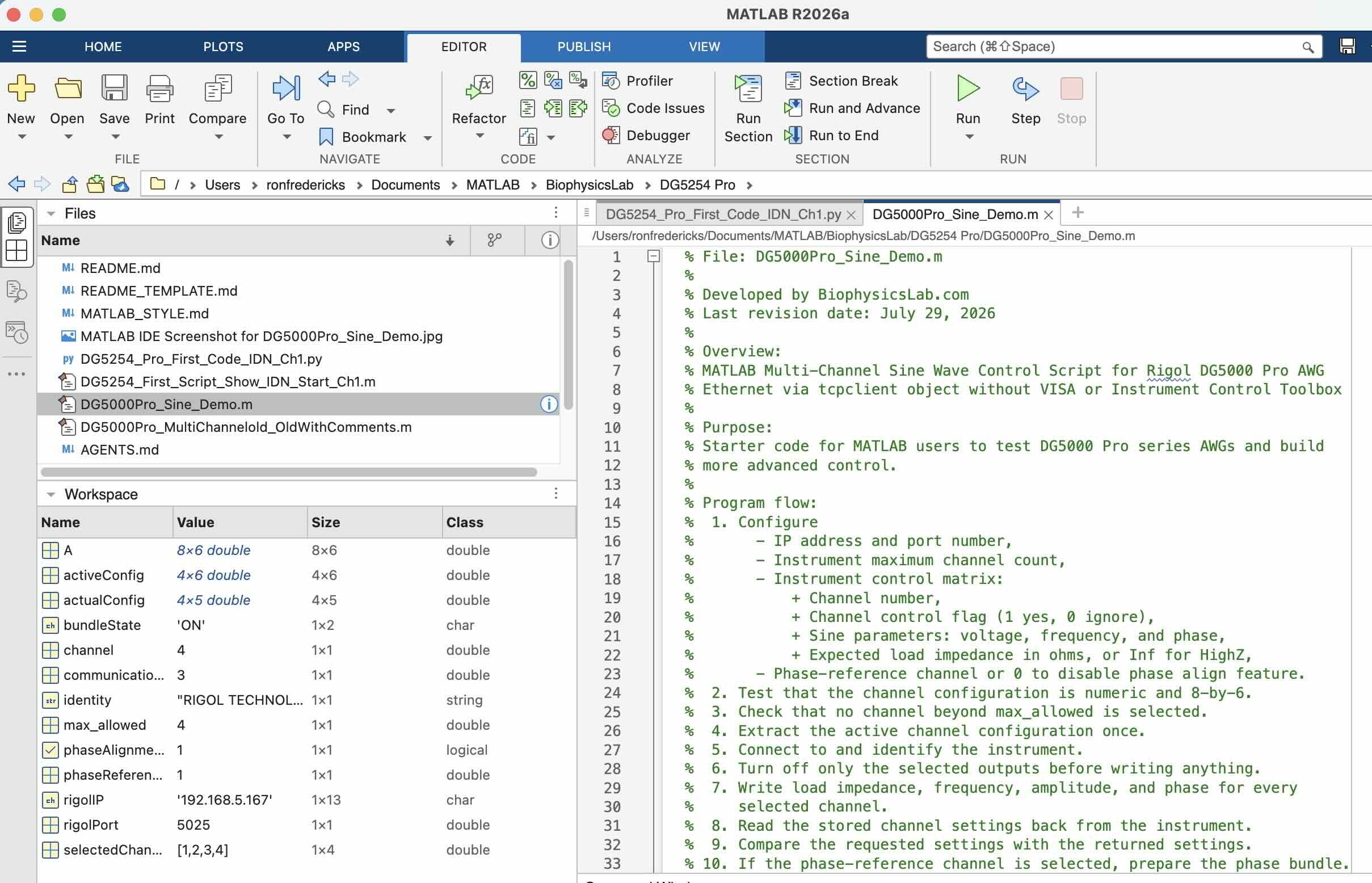
Representative MATLAB Command Window output
>> DG5000Pro_MultiChannel_Sine_Demo
Target: 192.168.5.167:5025
Channels to be changed: [1 2 3 4]
Phase alignment benchmark: Channel 1

Connected to: RIGOL TECHNOLOGIES,DG5254 Pro,DG5A286Mxxxxx,00.01.01

Channel 1 output disabled.
Channel 2 output disabled.
Channel 3 output disabled.
Channel 4 output disabled.
Channel 1 configured: 5000 Hz, 3 Vpp, 0 degrees, HighZ load.
Channel 2 configured: 5000 Hz, 3 Vpp, 45 degrees, HighZ load.
Channel 3 configured: 5000 Hz, 3 Vpp, 90 degrees, HighZ load.
Channel 4 configured: 5000 Hz, 3 Vpp, 135 degrees, HighZ load.
Read-back verified for 4 selected channels.
Phase benchmark: Channel 1
Channel 1 output enabled.
Channel 2 output enabled.
Channel 3 output enabled.
Channel 4 output enabled.
Bundled channel phases aligned.
Rigol TCP connection closed.The serial-number field in the identity string is intentionally redacted here. Your instrument will return its actual serial number.
Bundled-channel phase alignment
Rigol calls the phase reference the benchmark channel. The benchmark is automatically part of the bundled group. The script adds the other selected channels, enables the verified outputs, and then issues the one-shot phase-synchronize command. If only the benchmark channel is selected, the operation is valid but there is no second waveform to align. If phaseReferenceChannel is zero or names an unselected channel, alignment is skipped.
Channel 1 was the benchmark; Channels 2–4 were bundle members. Their programmed phases were 0°, 45°, 90°, and 135° before the one-shot alignment operation.
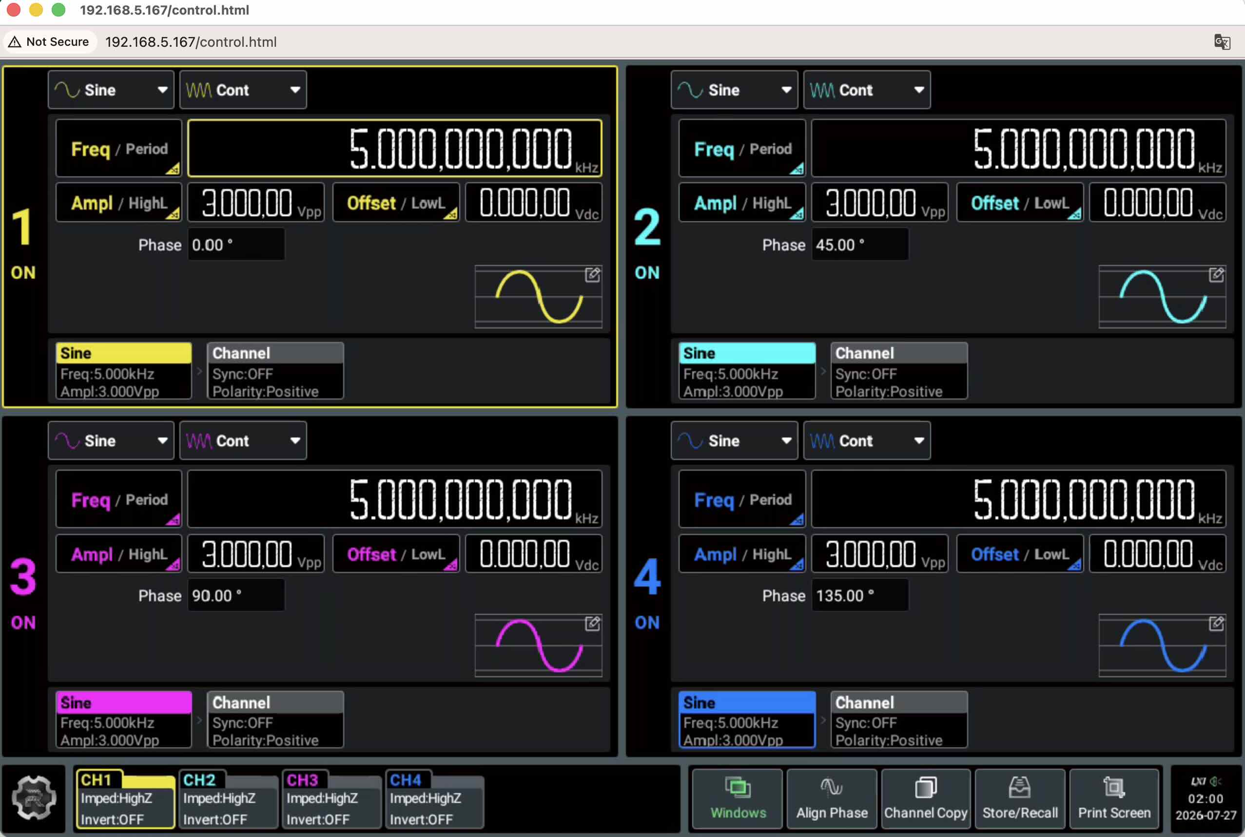
The web display shows each channel’s phase but does not visibly mark the phase-reference output in this view. Rigol’s programming guide calls that selected reference the benchmark channel. Earlier drafts called it the “bundled channel selected for control”; no different synchronization method is implied—the revised wording simply adopts Rigol’s terminology. See the DG5000 Pro Programming Guide for the synchronization commands.
Independent oscilloscope check
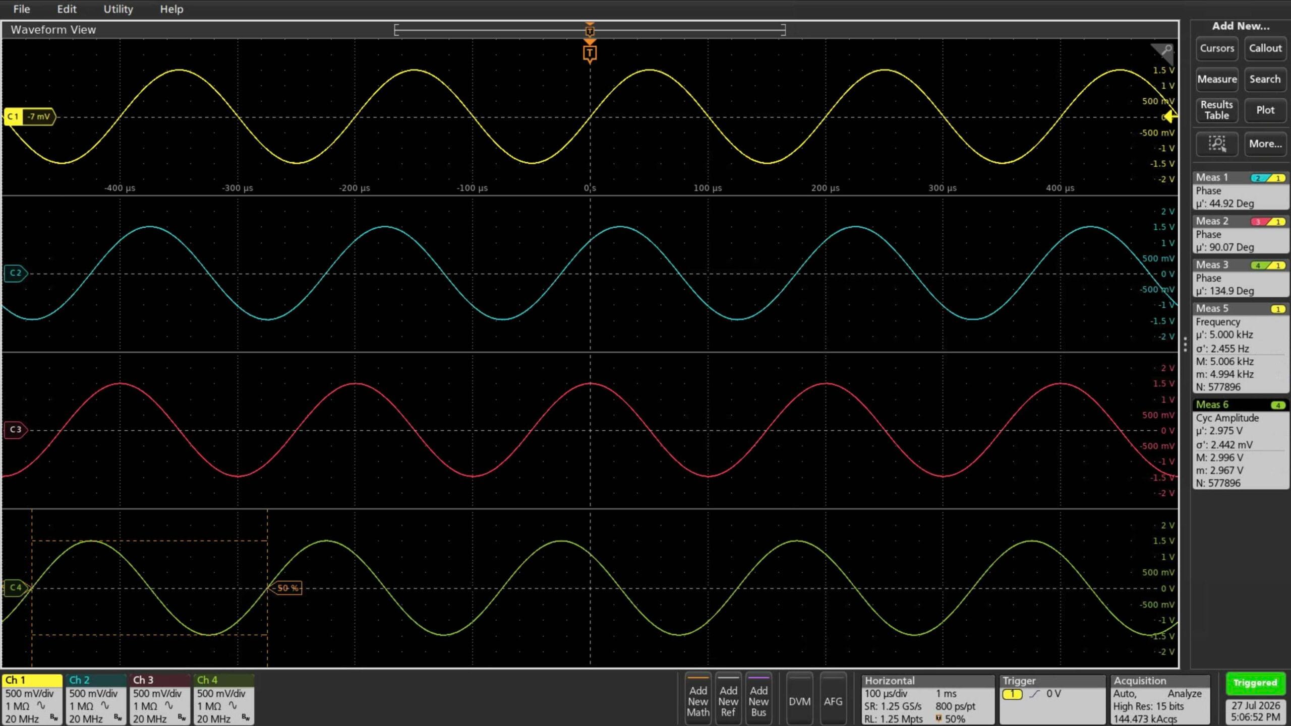
The Tektronix phase measurements were configured in the source order Ch2−Ch1, Ch3−Ch1, and Ch4−Ch1. Reversing the order changes a 45° lead into its modulo-360° equivalent, 315°; it does not mean the generator produced a different separation.
- Phase Ch2−Ch1: 44.92° average; 45° requested.
- Phase Ch3−Ch1: 90.07° average; 90° requested.
- Phase Ch4−Ch1: 134.9° average; 135° requested.
- Frequency: 5.000 kHz average; 5.000 kHz requested.
- Cycle amplitude: 2.975 V average; 3.000 Vpp requested.
Initially, the Peak-to-Peak measurement was configured to calculate one value for the entire acquired record. Its statistics therefore showed N′=1, even though the record contained many waveform cycles. I changed the badge to Amplitude and selected Calculate one measurement per: Cycle. After stopping acquisition, clearing the old statistics, and restarting, the scope accumulated one amplitude result for each cycle and produced meaningful multi-cycle statistics. I used AC coupling, 20 MHz bandwidth, 1 MΩ inputs, and Hi Res acquisition for this check. Tektronix documents the relevant measurement definitions in the 4/5/6 Series MSO Programmer Manual.
Small variations between Rigol settings and oscilloscope measurement badges are normal. Generator amplitude accuracy, scope vertical accuracy, input/load settings, bandwidth and acquisition mode, cable and termination effects, and each instrument’s calibration status all contribute to the observed value. A modest difference does not by itself show that either instrument is out of calibration; compare it with both instruments’ published specifications before investigating calibration.
Choosing a Human-Directed AI Coworker
Colin O’Flynn describes three practical levels of AI-assisted engineering:
- Conversational prompting: discuss a problem with an AI and manually transfer the useful results.
- AI coworker: discuss the work while the AI inspects and edits a bounded set of project files under user direction.
- Agentic execution: delegate a broader objective for the AI to pursue with greater autonomy.
For this project I chose the middle ground: discussion plus Codex working directly with a bounded project folder.
While the AI helped inspect files, refactor the scripts, preserve native errors, review terminology, build reusable project guidance, and prepare the article and download, I remained responsible for the hardware, measurements, engineering choices, and final publication decisions. That combination was more useful than isolated copy-and-paste prompts while keeping the experiment human-directed.
Both the waveform generator and oscilloscope are controlled from the host computer through TCP connections. With user-approved Computer Use enabled, Codex could also operate the Python and MATLAB environments directly, observe their results, and compare them with the instrument displays. The work still proceeded step by step under my control: I approved hardware-changing commands, confirmed oscilloscope measurements, and decided what entered the code and article.
Reference: Colin O’Flynn, “The Tireless Intern: LLM Coding Agents for Embedded Work—Using AI Speeds Security Tooling,” Circuit Cellar, Issue 432, July 2026, pp. 44–47. Issue 432 listing.
Using project context to guide advanced MATLAB coding
The file structure is itself a reusable AI-context system, not merely a collection of code. After extracting the download, a user can open its root folder with an AI coding coworker and ask it to read AGENTS.md before starting work. The files then supply project-specific grounding that influences how the AI understands the user, chooses MATLAB methods, edits files, verifies instrument behavior, and records lessons for the next project.
README.mdexplains the demonstrations, safety state, hardware scope, and entry points.AGENTS.mddefines the project purpose, collaboration rules, file-handling workflow, and reference routing.MATLAB_STYLE.mdteaches preferences such as logical indexing, array-oriented operations, explicit dimensions, appropriate loop use, and readable top-level scripts.references/MATLAB_REFERENCE_INDEX.mdroutes an AI to relevant pages in the external course notes instead of loading hundreds of pages for every task.references/MATLAB_SIGNATURE_METHODS.mdhighlights distinctive matrix, Fourier, signal-processing, statistics, fitting, and visualization methods that generic coding advice might overlook.retrospectives/preserves verified challenges, solutions, and transferable lessons without replacing the source code.templates/gives another user a starting structure for a different MATLAB/instrument project.
This can reasonably be described as teaching an AI coworker the author’s MATLAB style, but it is not model training or fine-tuning: the underlying model weights do not change. The reusable mechanism is contextual instruction and selective retrieval. Another user can keep these files, revise them for a new project, add their own methods and retrospectives, and pass the improved context forward.
How this relates to MATLAB Copilot and MCP
I began developing this project-owned context system because I wanted a transparent, portable way to control what an AI coding coworker learns about my MATLAB methods and each experiment. MathWorks now documents several related but distinct capabilities, so it is useful to separate them rather than treating “Copilot” and “MCP” as the same feature.
- MATLAB Copilot is an assistant integrated into the MATLAB desktop. It generates and explains code using MathWorks documentation, code examples, and relevant nearby or user-added code as context.
- MATLAB MCP Server is a tool bridge for external agents. It can start or connect to MATLAB, evaluate code, run files and tests, perform static code analysis, and identify installed toolboxes.
- MATLAB Agentic Toolkit combines the MCP connection with MathWorks-curated skills for idiomatic MATLAB workflows such as testing, debugging, code review, modernization, and app development.
- This download supplies user-owned project context: my coding preferences, course-note routing, instrument-specific behavior, safety decisions, verification evidence, and retrospectives. It works without MATLAB Copilot or MCP and can also complement either one.
For this experiment, direct project-folder access and user-approved Computer Use provided the middle-ground coworker model I wanted: the AI could edit the bounded files, operate Python and MATLAB, and observe results, while every hardware-changing step remained subject to my approval. An MCP connection could later replace some visual interaction with structured MATLAB tools without replacing the project-owned context.
Cycles of Efficiency™: From Context to Experimental Evidence
My original 2005 LectureMaker.com video-hosting services diagram for the EmbeddedComponents.com engineering marketplace presented Cycles of Efficiency™ as a lens that combined content, participation, distribution, and measurement to produce increasingly useful communication products. This laboratory project applies the same principle to engineering. Curated MATLAB knowledge informs the code; execution remains under human direction; instrument read-back and independent oscilloscope measurements provide evidence; and validated findings improve both the code and the reusable project context. The outputs from one experiment become inputs to the next cycle.
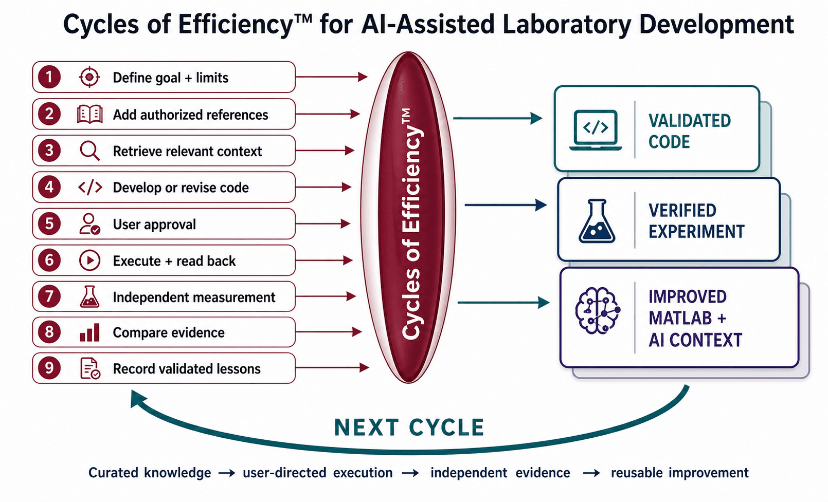
MathWorks states that end-user data submitted to MATLAB Copilot is used to fulfill requests and is not used to train AI models. Nearby or attached code is request context, which is conceptually closer to this project’s grounding approach than to model fine-tuning. See the MATLAB Copilot FAQ.
BiophysicsLab.com’s large course-note PDFs are deliberately not duplicated in the ZIP. The indexes and source links direct the AI to the relevant public document and pages when a task needs a specific method, figure, or explanation. To learn more about the MATLAB courses, follow Dr. Mike X Cohen at sincxpress.com.
- Master MATLAB Through Guided Problem Solving — Download PDF
- Signal Processing Problems Solved in MATLAB and Python — Download PDF
- Master the Fourier Transform and Its Applications Using MATLAB — Download PDF
- Complete Linear Algebra: Theory and Implementation in MATLAB and Python — Download PDF
Project Download

The project’s retrospective records transferable lessons rather than dumping the whole codebase into an AI prompt: keep demo controls visible, use logical indexing to select active rows, move repeated work into functions, distinguish read-back from analog validation, avoid hard-coded assumptions in friendly errors, and remove configuration machinery that obscures an educational example.