MATLAB Script for Tektronix Scope Plot and Measure
I present an updated 2-byte capture, plot, and measure script that follows current best practices using MATLAB’s Instrument Control Toolbox. My previous version was posted back in 2020. To start with, there is no VISA. Instead, the code is based on the TCP client object supported by the Tektronix instrument’s TCP/IP client service.
This script demonstrates how to use MATLAB’s Instrument Control Toolbox to communicate with a Tektronix MSO64B oscilloscope via TCP/IP. It captures, scales, plots, measures signal properties, displays results, and optionally saves the results.
MATLAB Script Overview
- Read Tektronix oscilloscope waveforms, plot results, show measurements, and save an image, the figure, or the workspace variables.
- The MATLAB script is coded to be easy to read, using code blocks and reusable functions. For example, all user controls are in one code block titled User Inputs.
- The script is designed to improve the value of oscilloscope data for research, engineering, and publication of results.
- Demonstrate communication with an oscilloscope using MATLAB’s tcpclient interface (no VISA) and scope’s Ethernet connection.
- Use the Oscilloscope SCPI CURve? command and the MATLAB readbinblock function to create a multi-channel plot with 2-byte (int16) data capture.
- Logic is included to produce meaningful color-coded plots with corresponding legend display.
- Logic is included to produce meaningful units for time and voltage in the plot and the legend.
- Optionally investigate the device under test (DUT) using plot data (experiment 1) and scope measurement badges (experiment 2).
- Modify the 2 existing experiments at a high level from the “User Inputs” code section.
- Review the “Measure (optional)” code section to design new experiments.
- Experiment 1 of 2 – use plot results:
- Use a flag to turn this experiment on or off; see variable do_experiment1_measurements.
- Show horizontal and vertical lines through maximum y value.
- Put a marker in the plot for the maximum y value.
- The legend displays the maximum voltage and corresponding time values below the marker.
- Experiment 2 of 2 – use scope measurement facilities:
- Use a flag to turn this experiment on or off; see variable do_experiment2_measurements.
- Use a table to define scope channels and their associated measurement parameters.
- Launch measurement badges on the oscilloscope for peak-2-peak, and frequency as examples of the many measurements available.
- Include measurements from any channel displayed on the scope – not just the channels plotted.
- For a list of all measurements available, refer to the Tektronix MSO 4,5,6 Programming Manual SCPI commands:
- DISplay:SELect:WAVEView1:SOUrce
- MEASUrement:ADDMEAS
- MEASUrement:MEAS
- Collect measurement badge values and optional statistics (min, max, std, population) based on trigger/acquisition mode.
- Use a flag to turn statistics on or off; see variable do_measure_statistics.
- Place collected badge measurement data into the plot legend.
- Optionally save the plot image, figure, and workspace for reuse.
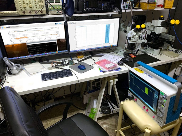
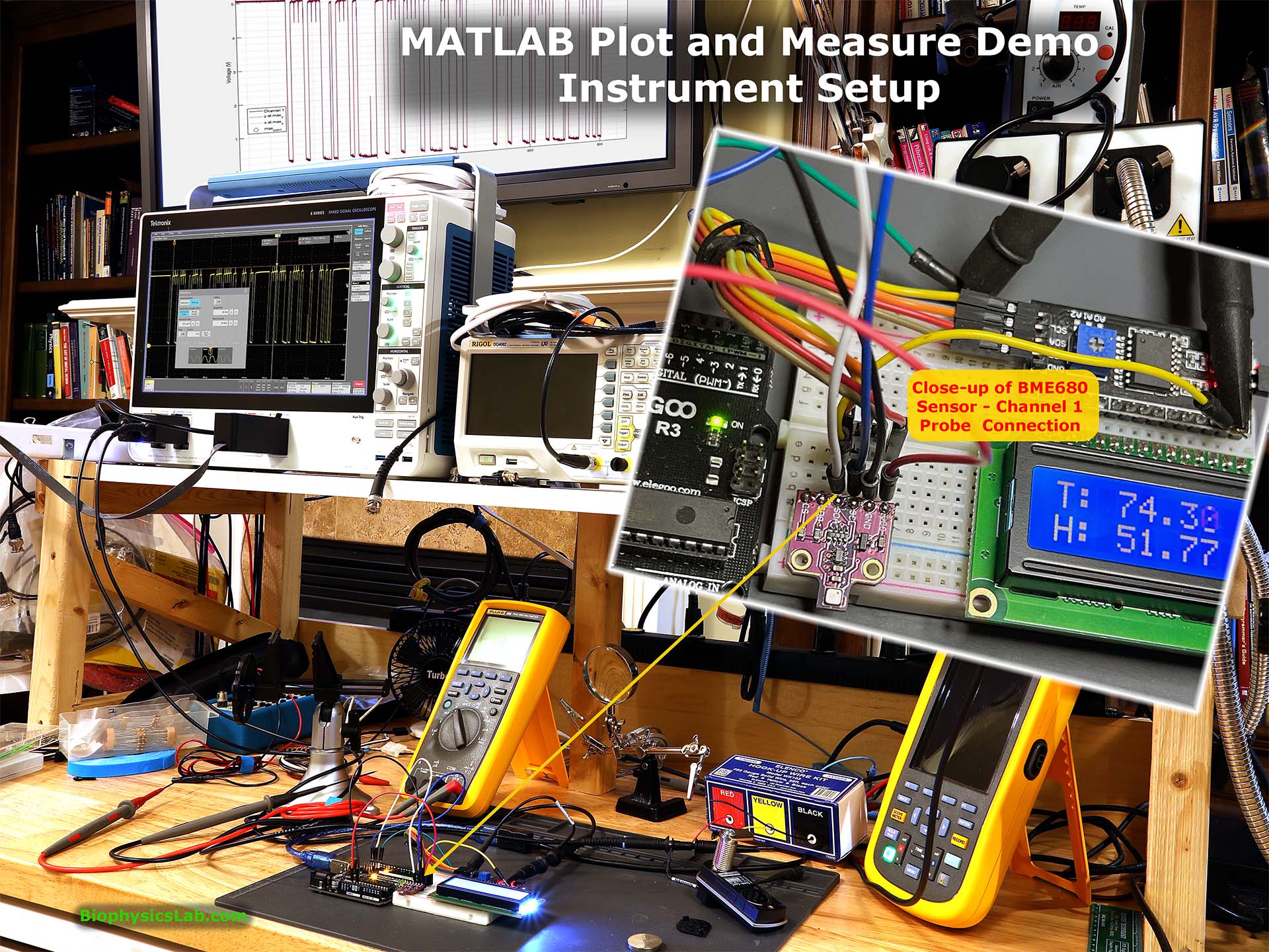
For this test setup, I used a single event trigger to capture the Serial Peripheral Interface (SPI) data output pin on a BME680 multifunction sensor controlled by an Arduino UNO R3.
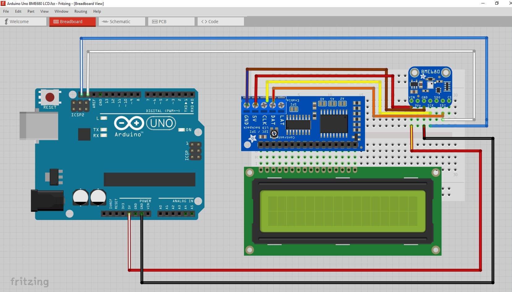
Fritzing Project Showing Andrino Uno Connections to BME680 Sensor
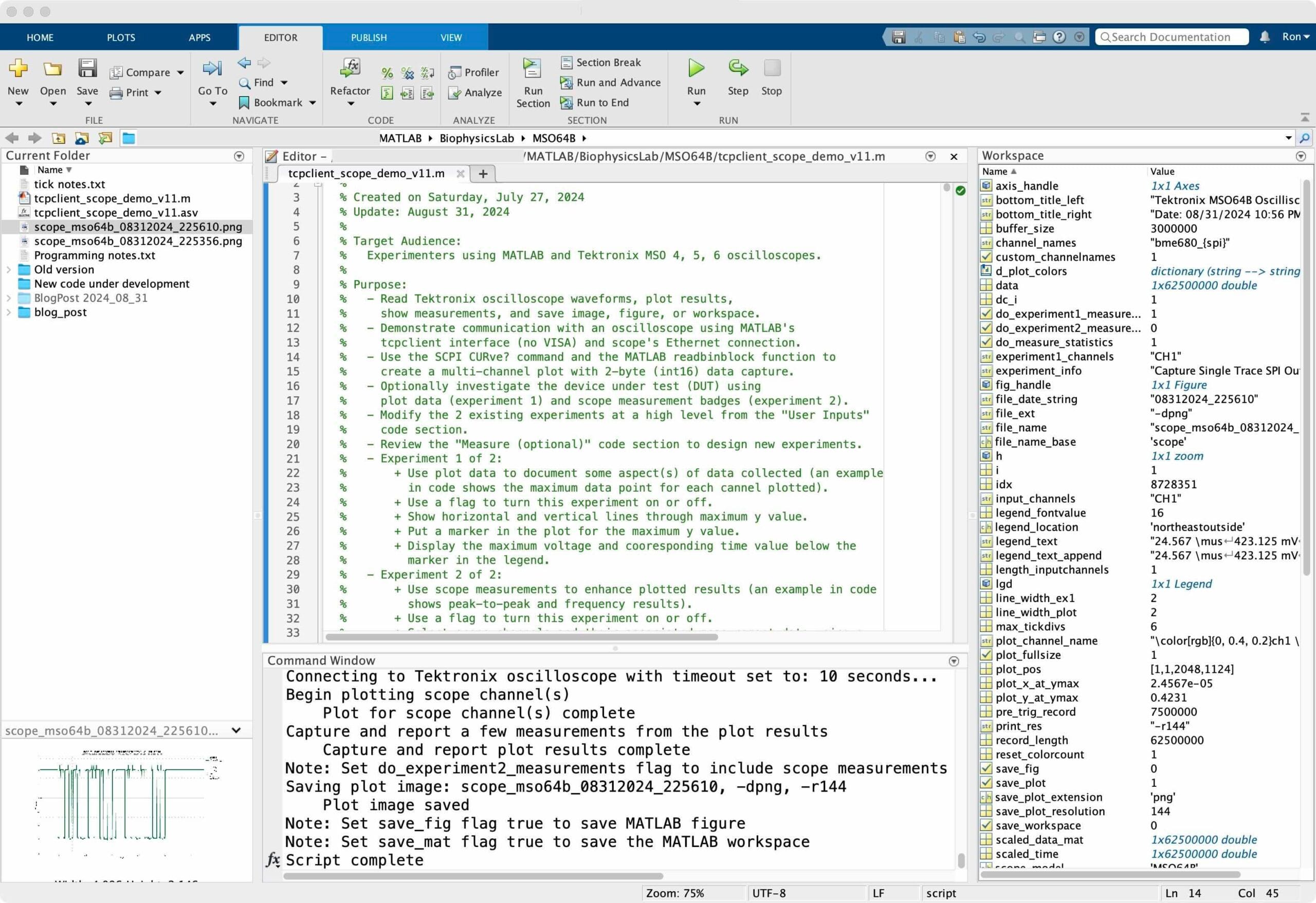
The MATLAB script editing environment shows some details about this script
Plots generated using this script
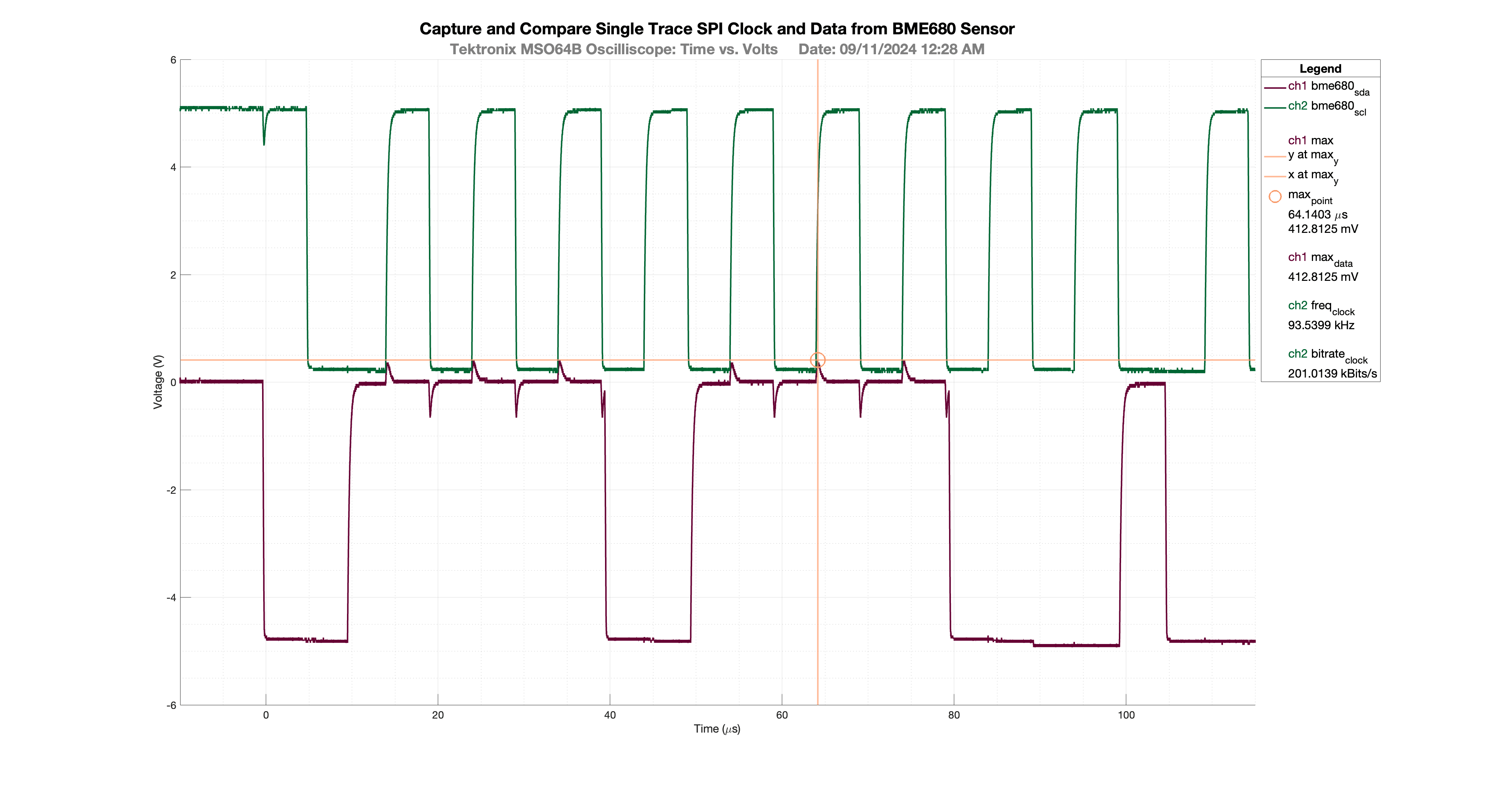
The script presented here shows how to capture a large single trace event from a Tektronix MSO64B oscilloscope. I suspect this script will work fine for any Tektronix scope from the MSO 4,5,6 family without modification. The plot shows the captured results automatically scaled to a user-friendly time scale:
- The magenta trace shows the scope’s channel 1 probe connected to the SPI data output from a BME680 sensor.
- The green trace shows the scope’s channel 2 probe connected to the BME680 SPI clock.
- The gold lines and markers are generated from the MATLAB plot data. In this case, the measurement shows the maximum data point, intersecting time, and voltage lines.
- The last 3 legend entries are measurements taken from the scope confirming the maximum data point is the same as the plot data point. Also the clock frequency and bitrate are shown using scope measurements as well.
- The legend is located outside the plot so much more data can be presented. The legend includes the automatic generation of a color-coded channel indicator and corresponding time and voltage values scaled to easy-to-read units. Statistics can also be displayed as part of the measurement badges during normal triggering.
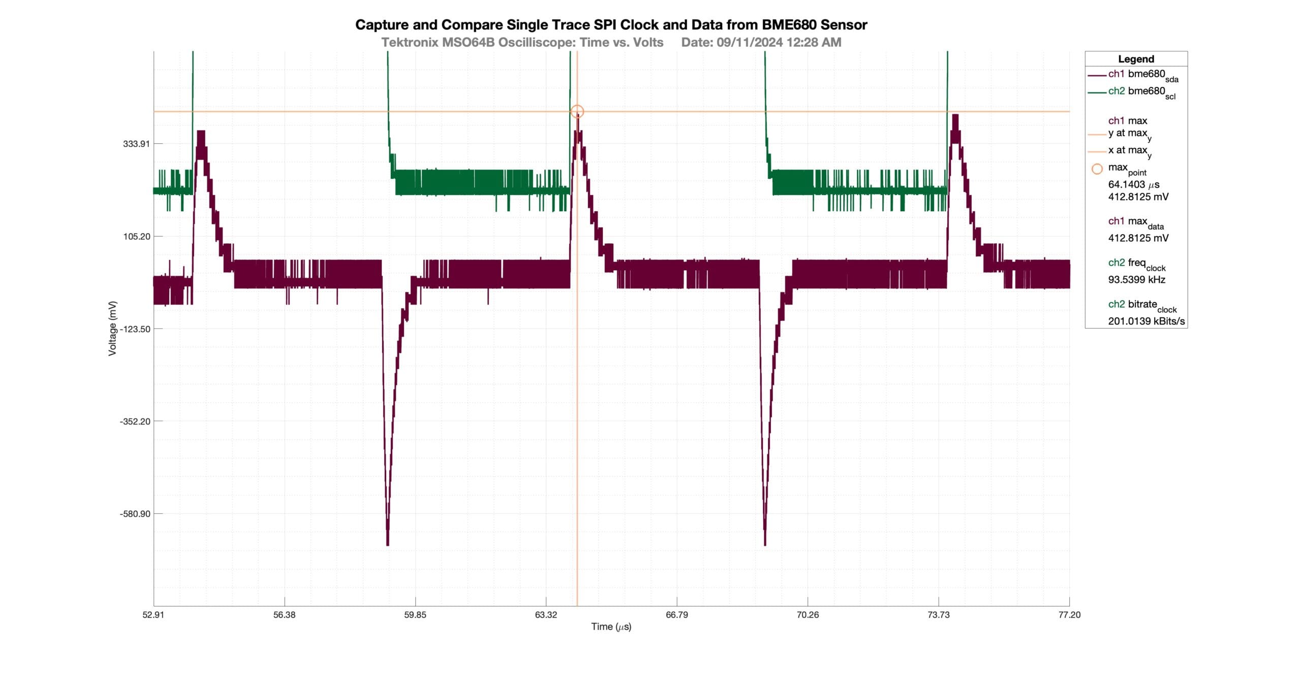
The figure above can be zoomed many times using the MATLAB Figure tool. When combined with the 2-byte data captured from the oscilloscope, the user can explore meaningful performance issues at a high magnification. Both the x and y-axis scales adjust automatically during the zoom process using a callback function from this script.
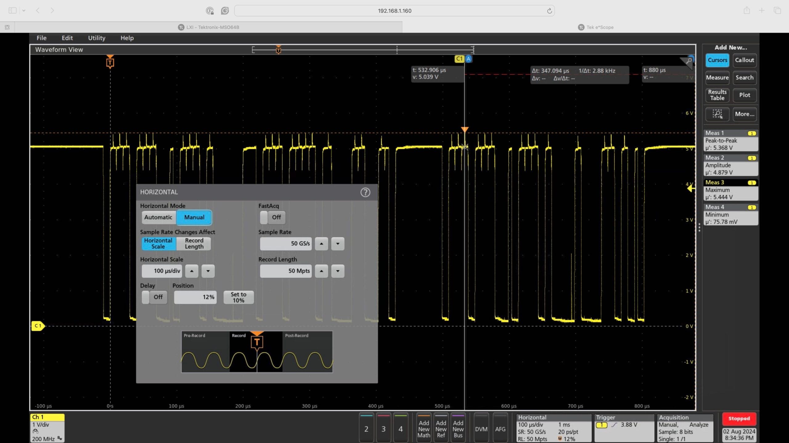
The eScope tool also works as a great diagnostic tool for new users connecting to scope via Ethernet using MATLAB’s tcpclient function. Note the measurement badges along the right margin. These badges were launched using this MATLAB script within the experiment 2 code block.
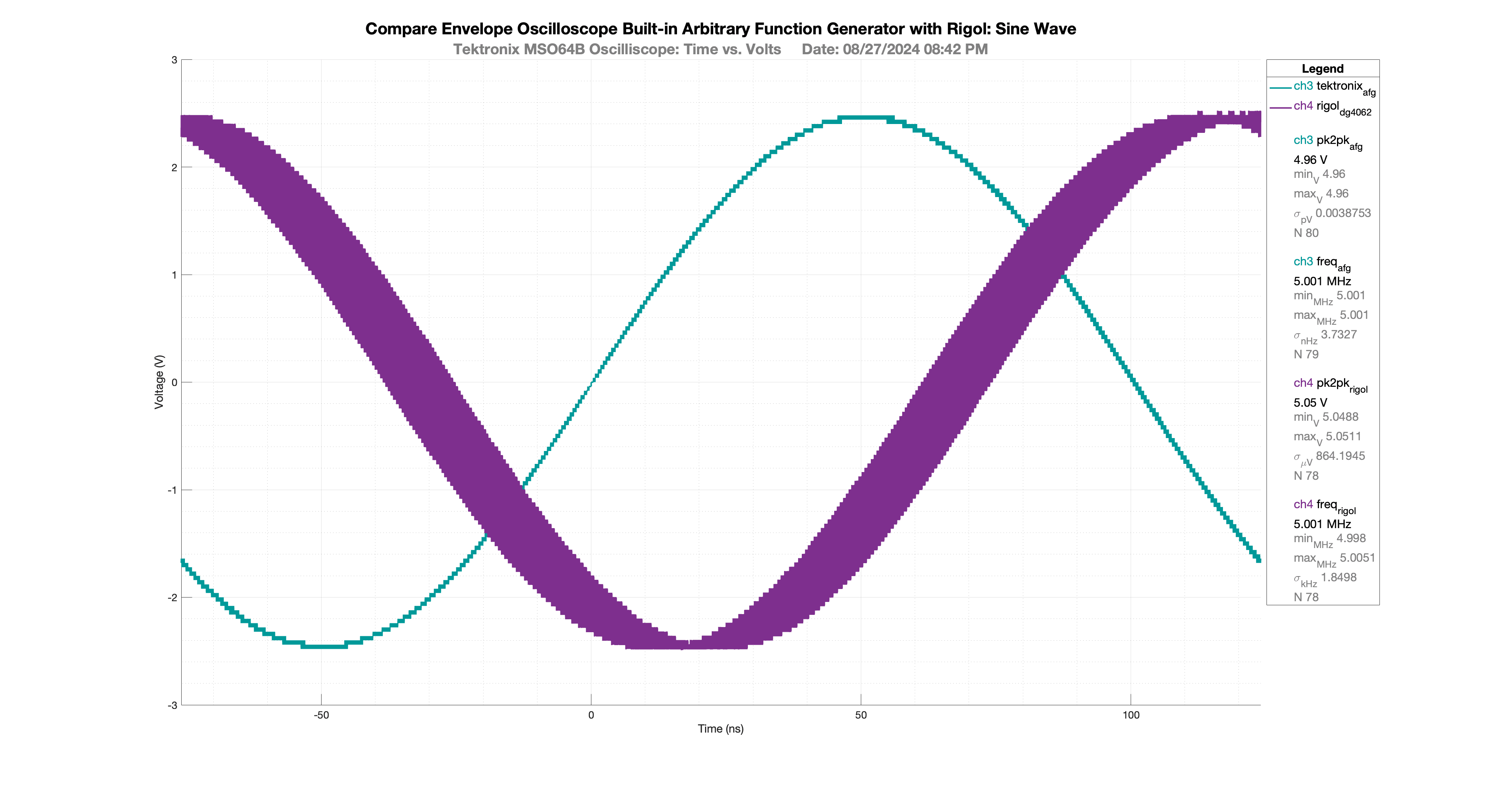
Plots Demonstrating Different Scope Acquisition Modes and Measurement Statistics
The results presented here are part of the code block controlled with the flag variable do_experiment2_measurements. The color-coded channels and measurement values improve documentation. The results and corresponding statistics help compare the two signal generators. In this case the frequency and the peak-to-peak values and standard deviation results show both instruments perform similarly at 45 MHz after a one hour warm-up period.
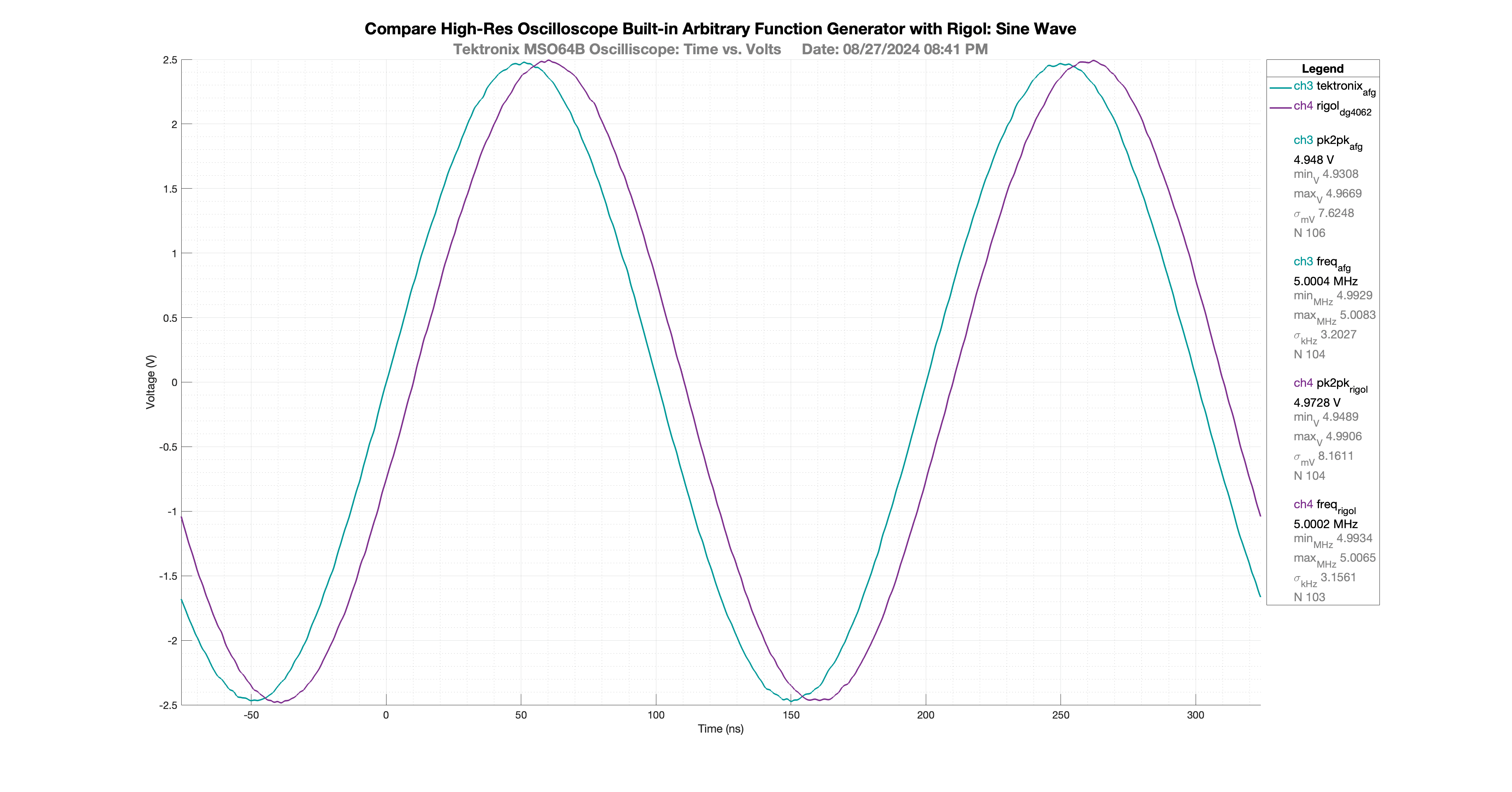
The oscilloscope envelope acquisition mode shows some jitter in the Rigol DG4062 arbitrary waveform generator (AWG) compared to the trigger-stabilized built-in Tektronix MSO64B arbitrary function generator (AFG).
MATLAB Script
Use this link to download the MATLAB script and selected sample images :

MATLAB Script for Tektronix Scope Plot and Measure
11
2026-05-26 09:52:02 GMT
View MATLAB script initial comments
%% File: tcpclient_scope_demo.m
%
% Created on Saturday, July 27, 2024
% Update: September 9, 2024
%
% Target Audience:
%   Experimenters using MATLAB and Tektronix MSO 4, 5, 6 oscilloscopes.
%   MATLAB versions tested: 2022b ... 2024a.
%   MATLAB versions 2022a and earlier would require several changes.
%
% Purpose:
%   - Read Tektronix oscilloscope waveforms, plot results,
%     show measurements, and save image, figure, or workspace.
%   - The MATLAB script is coded to be easy to read, using code blocks and
%     reusable functions. For example, all user controls are in one code block
%     titled User Inputs.
%   - The script is designed to improve the value of oscilloscope data for
%     research, engineering, and publication of results.
%   - Demonstrate communication with an oscilloscope using MATLAB's
%     tcpclient interface (no VISA) and scope's Ethernet connection.
%   - Use the SCPI CURve? command and the MATLAB readbinblock function to
%     create a multi-channel plot with 2-byte (int16) data capture.
%   - Logic is included to produce meaningful color-coded plots with
%     corresponding legend display.
%   - Logic is included to produce meaningful units for time and voltage in
%     the plot and the legend. During plot zoom, units extend to the limit of
%     the scope's timeline increment (8.0e-11 seconds for example).
%   - Optionally investigate the device under test (DUT) using
%     plot data (experiment 1) and scope measurement badges (experiment 2).
%   - Modify the 2 existing experiments at a high level from the "User Inputs"
%     code section.
%   - Review the "Measure (optional)" code section to design new experiments.
%   - Experiment 1 of 2 - use plot results:
%       + Use a flag to turn this experiment on or off;
%         see variable do_experiment1_measurements.
%       + Show horizontal and vertical lines through maximum y value.
%       + Put a marker in the plot for the maximum y value.
%       + The legend displays the maximum voltage and corresponding time values
%         below the marker.
%   - Experiment 2 of 2 - use scope measurement facilities:
%       + Use a flag to turn this experiment on or off;
%         see variable do_experiment2_measurements.
%       + Use a table to define scope channels and their associated measurement
%         parameters.
%       + Launch measurement badges on the oscilloscope for peak-2-peak, and
%         frequency as examples of the many measurements available.
%       + Include measurements from any channel displayed on scope - not
%         just the channels plotted in MATLAB.
%       + For a list of all measurements available, refer to the Tektronix
%         MSO 4,5,6 Programming Manual SCPI commands:
%           DISplay:SELect:WAVEView1:SOUrce
%           MEASUrement:ADDMEAS
%           MEASUrement:MEAS
%       + Collect measurement badge values and optional statistics
%         (min, max, std, population) based on trigger/acquisition mode.
%       + Use a flag to turn statistics on or off.
%       + Place collected badge measurement data into the plot legend.
%   - Optionally save the plot image, figure, and workspace for reuse.
%
% Author: BiophysicsLab.com
%
% Discussion Web Page:
%   https://www.biophysicslab.com/2024/08/31/matlab-script-for-tektronix-scope-plot-and-measure/
%
% Products Used:
%   Tektronix 6 Series B MSO Mixed Signal Oscilloscope
%   Model MSO64B with Firmware Updated to FV:2.8.1.1496 now to FV:2.10.5.1825
%   https://www.tek.com/en/products/oscilloscopes/6-series-mso
%
%   MATLAB Instrument Control Toolbox (ICT)
%   Control test and measurement instruments and communicate with computer peripherals
%   MATLAB Version R2023b with Instrument Control Toolbox (ICT)
%   https://www.mathworks.com/products/instrument.html
%   https://www.mathworks.com/help/instrument/transition-your-code-to-tcpclient-interface.html
%
%   Mac Studio M1 Ultra (Apple Silicon) MacOS Sonoma Version: 14.5
%   https://www.apple.com/mac-studio/
%
% Parameters used for accurate time and voltage plotting:
%   ymult > SCPI command: 'WFMOutpre:YMULT?'
%   yzero > SCPI command: 'WFMOutpre:YZERO?'
%   yoff > SCPI command: 'WFMOutpre:YOFF?'
%   xincr > SCPI command: 'WFMOutpre:XINCR?'
%   xzero > SCPI command: 'WFMOutpre:XZERO?'
%   pre_trig_record > SCPI command: 'WFMOutpre:PT_OFF?'
%
%   SCPI command reference:
%       https://www.tek.com/en/sitewide-content/manuals/4/5/6/4-5-6-series-mso-programmer-manual
%
% Useful Discussion Threads:
%
%   MATLAB Script for Tektronix Scope Plot and Measure
%   https://www.biophysicslab.com/2024/08/01/matlab-script-for-tektronix-scope-plot-and-measure/
%
%   MATLAB ICT: MDO Simple Plot
%   https://forum.tek.com/viewtopic.php?f=580&t=141809
%
%   MATLAB Oscilloscope App
%   https://www.mathworks.com/matlabcentral/fileexchange/69847-oscilloscope-app
%
%   Python MSO64 2-byte read binary waveform example
%   https://forum.tek.com/viewtopic.php?f=580&t=142410
%
%   Python: MDO Simple Plot
%   https://forum.tek.com/viewtopic.php?t=138684
%
%   MSO6 read Meas with SCPI command (eg PYTHON)
%   https://forum.tek.com/viewtopic.php?t=142486
%
% Code sections:
%   User Inputs
%   Initialize Instrument
%   Instrument Control
%   Get Waveform(s)
%   Plot
%   Measure (optional)
%   Save (optional)
%   Close Session
%   Reusable Functions
%
% Reusable Functions:
%   function byte = get_byteFcn(x)
%   function result_flag = is_scipi_nan(val)
%   function [scale_exp, scale_txt] = scale_resultsFcn(values, top_units)
%   function color = get_plotColorFcn(reset_colorcount)
%   function chan_txt  = get_channelNameFcn(chan)
%   function sesr = test_sesrFcn(scope, code_msg)
%   function scope_model = get_identityFcn(scope, scope_vendor)
%   function channel_used = is_channelFcn(scope, chan)
%   function scope_trigger = get_triggerFcn(scope)
%   function zoomCallbackFcn(obj,evd)
%   function [new_xyticks_rnd, cell_labels, errFlg] = scale_ticksFcn(xyround, xyround_lmt, new_xylim, max_xytickdivs)
%   function adjacent_equal = adjacentEqualFcn(a, tol)
%   function zoomErrorFcn()
%   function legend_text_append = makeBadgeFcn(title, value, units, color)
%   function num_zeros = nearZeroFcn(num, tol)
%   function rgbstr = hex2rgbStringFcn(hex)
%   function [ rgb ] = hex2rgb(hex,range) ** MATLAB Central File Exchange **
%
% TODO(s):
%   - Convert this code to an object oriented program (OOP):
%       + Convert some User Input code section into a constructor
%       + Use getter/setter methods to change experiment input code
%       + Instrument class
%       + Plot class
%       + Experiment class(s)
%       + Convert functions to methods
%   - MATHx and REFx scope channels require additional programming to plot.
%   - Add a stacked option for plotting each channel
%       https://www.mathworks.com/support/search.html/answers/1573168-adding-event-markers-to-imported-eeg-data-stacked-plot.html
%   - Feature: With the existing workspace loaded, run this program again
%     without instrument capture, allowing new plot measurements and formatting
%     with the instrument turned off.


%% User Inputs
% User Input Sections:
%   - Controls for oscilloscope
%   - Controls for saving data: image, figure, workspace mat
%   - Controls for plot
%   - Controls for lab experiments
%       + plot max point
%       + scope measurements from Tektronix measurement badges
References
- SCPI reference and programmer guide for Tektronix MSO 4,5,6 osillocopes: https://www.tek.com/en/sitewide-content/manuals/4/5/6/4-5-6-series-mso-programmer-manual
- Standard Commands for Programmable Instruments (SCPI): https://www.ivifoundation.org/downloads/SCPI/scpi-99.pdf
- MATLAB Instrument Control Toolbox tcpclient interface: https://www.mathworks.com/help/instrument/transition-your-code-to-tcpclient-interface.html
- My MATLAB programming notes: https://www.biophysicslab.com/portfolio/matlab-projects/
- My previous post on MATLAB oscilloscope data capture: https://www.biophysicslab.com/2020/10/11/matlab-2-byte-data-capture-from-tektronix-mso64-oscilloscope/
- My prior research using the Arduino with BME680 Sensor: https://www.biophysicslab.com/2022/10/05/arduino-circuit-design-using-bme680-sensor/